16. XGBoost

XGBoost, or eXtreme Gradient Boosting, is gradient boosting library. Although scikit-learn has several boosting algorithms available, XGBoost’s implementations are parallelized and takes advantage of GPU computing. A few of the types of learners XGBoost has include gradient boosting for regression, classification and survival analysis (e.g. Accelerated Failure Time AFT). There are no shortages of boosting libraries; here’s a few more.

• LightGBM

• CatBoost

16.1. Regression

Let’s see how XGBoost works on regression problems by first simulating data.

import numpy as np
import random
from sklearn.datasets import make_regression

random.seed(37)
np.random.seed(37)

X, y = make_regression(**{
    'n_samples': 1000,
    'n_features': 10,
    'n_targets': 1,
    'bias': 5.3,
    'random_state': 37
})

print(f'X shape = {X.shape}, y shape {y.shape}')

X shape = (1000, 10), y shape (1000,)

We will split the generated data into training and testing sets.

from sklearn.model_selection import train_test_split

X_train, X_test, y_train, y_test = train_test_split(X, y, test_size=0.2, random_state=37)

print(X_train.shape, y_train.shape)
print(X_test.shape, y_test.shape)

(800, 10) (800,)
(200, 10) (200,)

The XGBRegressor class is used to learn a boosted regression model. Note that the objective is specified to reg:squarederror. A list of objectives is available. Here, we specify only 10 estimators.

import xgboost as xgb

model = xgb.XGBRegressor(objective='reg:squarederror', n_estimators=10, seed=37)
model.fit(X_train, y_train)

XGBRegressor(base_score=0.5, booster='gbtree', colsample_bylevel=1,
             colsample_bynode=1, colsample_bytree=1, gamma=0, gpu_id=-1,
             importance_type='gain', interaction_constraints='',
             learning_rate=0.300000012, max_delta_step=0, max_depth=6,
             min_child_weight=1, missing=nan, monotone_constraints='()',
             n_estimators=10, n_jobs=12, num_parallel_tree=1, random_state=37,
             reg_alpha=0, reg_lambda=1, scale_pos_weight=1, seed=37,
             subsample=1, tree_method='exact', validate_parameters=1,
             verbosity=None)

We will measure the performance of the model using mean absolute error (MAE) and root mean squared error (RMSE).

from sklearn.metrics import mean_squared_error, mean_absolute_error

y_pred = model.predict(X_test)

mae = mean_absolute_error(y_test, y_pred)
rmse = np.sqrt(mean_squared_error(y_test, y_pred))

print(mae)
print(rmse)

35.00964208044854
44.165107049077356

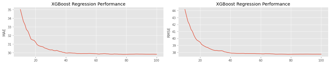
As you increase the number of estimators, the performance should increase, as measured by MAE and RMSE. There is a point of diminishing returns, however.

import pandas as pd

def get_performance(n_estimators):
    model = xgb.XGBRegressor(objective='reg:squarederror', n_estimators=n_estimators, seed=37)
    model.fit(X_train, y_train)

    y_pred = model.predict(X_test)

    mae = mean_absolute_error(y_test, y_pred)
    rmse = np.sqrt(mean_squared_error(y_test, y_pred))
    return {'mae': mae, 'rmse': rmse}

n_estimators = list(range(10, 101, 1))
results = pd.DataFrame([get_performance(n) for n in n_estimators], index=n_estimators)

import matplotlib.pyplot as plt

plt.style.use('ggplot')

fig, axes = plt.subplots(1, 2, figsize=(15, 3))

_ = results.mae.plot(ax=axes[0])
_ = results.rmse.plot(ax=axes[1])

axes[0].set_title('XGBoost Regression Performance')
axes[1].set_title('XGBoost Regression Performance')

axes[0].set_ylabel('MAE')
axes[1].set_ylabel('RMSE')

plt.tight_layout()

16.2. Classification

Let’s turn our attention to using XGBoost for classification by generating data for a classification problem.

from sklearn.datasets import make_classification

X, y = make_classification(**{
    'n_samples': 2000,
    'n_features': 20,
    'n_informative': 10,
    'n_redundant': 0,
    'n_repeated': 0,
    'n_classes': 2,
    'random_state': 37
})

print(f'X shape = {X.shape}, y shape {y.shape}')

X shape = (2000, 20), y shape (2000,)

We will split the data into training and testing sets.

X_train, X_test, y_train, y_test = train_test_split(X, y, test_size=0.2, random_state=37)

print(X_train.shape, y_train.shape)
print(X_test.shape, y_test.shape)

(1600, 20) (1600,)
(400, 20) (400,)

The input data must be transformed from numpy arrays into DMatrix.

dtrain = xgb.DMatrix(X_train, y_train)
dtest = xgb.DMatrix(X_test, y_test)

print(dtrain.num_row(), dtrain.num_col())
print(dtest.num_row(), dtest.num_col())

1600 20
400 20

Now we are ready to learn a classification model with XGBoost.

param = {
    'max_depth':2,
    'eta':1,
    'objective':'binary:logistic',
    'eval_metric': 'logloss',
    'seed': 37
}
num_round = 20

model = xgb.train(param, dtrain, num_round)

We will measure the performance of the model using Area Under the Curve (the Receiver Operating Characteristic curve) and the Average Precision Score.

from sklearn.metrics import roc_auc_score, average_precision_score

y_pred = model.predict(dtest)

auc = roc_auc_score(y_test, y_pred)
aps = average_precision_score(y_test, y_pred)

print(auc)
print(aps)

0.951115116017121
0.9450649144817633

16.3. Survival

Let’s see how survival regression works with XGBoost. Let’s sample some data.

X, y = make_regression(**{
    'n_samples': 1000,
    'n_features': 4,
    'n_targets': 0,
    'random_state': 37
})

coef = np.array([2.0, -1.0, 3.5, 4.4])
baseline = np.e / np.power(1 + np.e, 2.0)
y = np.exp(-X.dot(coef)) * baseline

print(f'X shape = {X.shape}, y shape {y.shape}, coef shape = {coef.shape}')

X shape = (1000, 4), y shape (1000,), coef shape = (4,)

Here, we will split the data into training and testing sets.

X_train, X_test, y_train, y_test = train_test_split(X, y, test_size=0.2, random_state=37)

print(X_train.shape, y_train.shape)
print(X_test.shape, y_test.shape)

(800, 4) (800,)
(200, 4) (200,)

Let’s turn the inputs into the appropriate format. Note that we do not supply the duration into the DMatrix but set the lower and upper bound using the set_float_info() method.

dtrain = xgb.DMatrix(X_train)
dtest = xgb.DMatrix(X_test)

dtrain.set_float_info('label_lower_bound', y_train)
dtest.set_float_info('label_lower_bound', y_test)

dtrain.set_float_info('label_upper_bound', y_train)
dtest.set_float_info('label_upper_bound', y_test)

print(dtrain.num_row(), dtrain.num_col())
print(dtest.num_row(), dtest.num_col())

800 4
200 4

The following shows how to specify a survival model with AFT.

params = {
    'objective': 'survival:aft',
    'eval_metric': 'aft-nloglik',
    'aft_loss_distribution': 'logistic',
    'aft_loss_distribution_scale': 1.0,
    'tree_method': 'exact',
    'learning_rate': 0.05,
    'max_depth': 5
}
model = xgb.train(params, dtrain, num_boost_round=40, evals=[(dtrain, 'train')])

[0]     train-aft-nloglik:2.58474
[1]     train-aft-nloglik:2.13443
[2]     train-aft-nloglik:1.76805
[3]     train-aft-nloglik:1.51551
[4]     train-aft-nloglik:1.30791
[5]     train-aft-nloglik:1.15456
[6]     train-aft-nloglik:1.01593
[7]     train-aft-nloglik:0.90408
[8]     train-aft-nloglik:0.80288
[9]     train-aft-nloglik:0.71937
[10]    train-aft-nloglik:0.64163
[11]    train-aft-nloglik:0.57327
[12]    train-aft-nloglik:0.51536
[13]    train-aft-nloglik:0.46241
[14]    train-aft-nloglik:0.41428
[15]    train-aft-nloglik:0.37151
[16]    train-aft-nloglik:0.33085
[17]    train-aft-nloglik:0.29569
[18]    train-aft-nloglik:0.26403
[19]    train-aft-nloglik:0.23559
[20]    train-aft-nloglik:0.20816
[21]    train-aft-nloglik:0.18294
[22]    train-aft-nloglik:0.16056
[23]    train-aft-nloglik:0.13968
[24]    train-aft-nloglik:0.11968
[25]    train-aft-nloglik:0.10160
[26]    train-aft-nloglik:0.08428
[27]    train-aft-nloglik:0.06922
[28]    train-aft-nloglik:0.05431
[29]    train-aft-nloglik:0.04075
[30]    train-aft-nloglik:0.02782
[31]    train-aft-nloglik:0.01519
[32]    train-aft-nloglik:0.00409
[33]    train-aft-nloglik:-0.00611
[34]    train-aft-nloglik:-0.01670
[35]    train-aft-nloglik:-0.02580
[36]    train-aft-nloglik:-0.03482
[37]    train-aft-nloglik:-0.04267
[38]    train-aft-nloglik:-0.05033
[39]    train-aft-nloglik:-0.05770

Below, we evaluate the model using the c-index.

from itertools import combinations

def get_status(p1, p2):
    x1, y1 = p1[0], p1[1]
    x2, y2 = p2[0], p2[1]

    r = (y2 - y1) * (x2 - x1)

    if r > 0:
        return 1
    elif r < 0:
        return -1
    else:
        return 0

y_pred = model.predict(dtest)
pairs = combinations([(y_t, y_p) for y_t, y_p in zip(y_test, y_pred)], 2)
results = [get_status(p1, p2) for p1, p2 in pairs]
c = sum([1 for r in results if r == 1])
n = len(results)
print(c / n)

0.9332160804020101

The c-index of the predictions from the training is as expected; it’s higher than the testing set.

y_pred = model.predict(dtrain)

pairs = combinations([(y_t, y_p) for y_t, y_p in zip(y_train, y_pred)], 2)
results = [get_status(p1, p2) for p1, p2 in pairs]
c = sum([1 for r in results if r == 1])
n = len(results)
print(c / n)

0.9664893617021276