14. MLflow

MLflow is YALF (yet another logging framework) for data science experiments. You can log just about anything important from your experiments including stats, performances, parameters, figures, intermediary results, models, etc. Many different data science frameworks (or flavors) are supported, including Scikit-Learn, PyTorch, XGBoost, etc. Since you can log the models (or persist the models), you can even use MLflow to depersist these models and make predictions! Let’s see how MLflow works.

Here, we create a classification problem with the typical Xy data shapes.

from sklearn.datasets import make_classification
import pandas as pd

def get_Xy():
    n_features = 10
    X, y = make_classification(**{
        'n_samples': 2000,
        'n_features': n_features,
        'n_informative': 2,
        'n_redundant': 2,
        'n_repeated': 0,
        'n_classes': 2,
        'n_clusters_per_class': 1,
        'random_state': 37
    })

    cols = [f'x{i}' for i in range(n_features)]
    return pd.DataFrame(X, columns=cols), y

X, y = get_Xy()
X.shape, y.shape, X.columns

((2000, 10),
 (2000,),
 Index(['x0', 'x1', 'x2', 'x3', 'x4', 'x5', 'x6', 'x7', 'x8', 'x9'], dtype='object'))

Then, we split Xy into training X_tr, y_tr and testing X_te, y_te.

from sklearn.model_selection import train_test_split

X_tr, X_te, y_tr, y_te = train_test_split(X, y, test_size=0.3, random_state=37)

X_tr.shape, y_tr.shape, X_te.shape, y_te.shape

((1400, 10), (1400,), (600, 10), (600,))

We are going to fit a logistic regression model and look at the performances for both training and testing sets.

from sklearn.linear_model import LogisticRegression
from sklearn.model_selection import GridSearchCV, StratifiedKFold
from sklearn.metrics import average_precision_score, roc_auc_score, precision_score, recall_score, f1_score
import numpy as np

def get_model():
    estimator = LogisticRegression(**{
        'solver': 'saga',
        'penalty': 'l2',
        'random_state': 37,
        'max_iter': 1_000
    })

    cv = StratifiedKFold(**{
        'n_splits': 5,
        'shuffle': True,
        'random_state': 37
    })

    model = GridSearchCV(**{
        'estimator': estimator,
        'cv': cv,
        'param_grid': {
            'penalty': ['l1', 'l2'],
            'C': [0.01, 0.5, 0.7, 0.9]
        },
        'scoring': {
            'auc': 'roc_auc',
            'apr': 'average_precision'
        },
        'verbose': 5,
        'refit': 'apr',
        'error_score': np.NaN,
        'n_jobs': -1
    })

    return model

def get_performances(X_tr, y_tr, X_te, y_te, model):
    y_tr_pred = model.predict(X_tr)
    y_te_pred = model.predict(X_te)

    pre_tr = precision_score(y_tr, y_tr_pred)
    pre_te = precision_score(y_te, y_te_pred)

    rec_tr = recall_score(y_tr, y_tr_pred)
    rec_te = recall_score(y_te, y_te_pred)

    f1_tr = f1_score(y_tr, y_tr_pred)
    f1_te = f1_score(y_te, y_te_pred)

    y_tr_prob = model.predict_proba(X_tr)[:,1]
    y_te_prob = model.predict_proba(X_te)[:,1]

    auc_tr = roc_auc_score(y_tr, y_tr_prob)
    auc_te = roc_auc_score(y_te, y_te_prob)

    aps_tr = average_precision_score(y_tr, y_tr_prob)
    aps_te = average_precision_score(y_te, y_te_prob)

    perf_metrics = {
        'pre_tr': pre_tr,
        'pre_te': pre_te,
        'rec_tr': rec_tr,
        'rec_te': rec_te,
        'f1_tr': f1_tr,
        'f1_te': f1_te,
        'auc_tr': auc_tr,
        'auc_te': auc_te,
        'aps_tr': aps_tr,
        'aps_te': aps_te
    }

    return perf_metrics

Here is where MLflow comes in. As we progress through our experimental procedure, we can log nearly anything we want about the experiment. The tracking_uri points to the MLflow server and the experiment_name is the name of your experiment (many models can map to the same experiment, such as a set of random forest, logistic regression and gradient boosting models). Below, we log

• the model,

• the performances of the model,

• the cross-validation results of the hyperparameter tuning grid search, and

• a few graphs to visualize the data.

import mlflow
from mlflow.exceptions import MlflowException
from mlflow.models.signature import infer_signature
import matplotlib.pyplot as plt
import seaborn as sns

plt.style.use('ggplot')

experiment_name = 'test1'

if not mlflow.get_experiment_by_name(experiment_name):
    try:
        mlflow.create_experiment(experiment_name)
    except MlflowException as ex:
        print(f'{ex}')

tracking_uri = 'http://localhost:5001'

mlflow.set_tracking_uri(tracking_uri)
mlflow.set_experiment(experiment_name)

with mlflow.start_run() as run:
    model = get_model()
    model.fit(X_tr, y_tr)

    signature = infer_signature(X_tr, model.predict_proba(X_tr))
    mlflow.sklearn.log_model(model, 'model', signature=signature)
    mlflow.log_params(model.best_params_)

    perf_metrics = get_performances(X_tr, y_tr, X_te, y_te, model)
    mlflow.log_metrics(perf_metrics)

    pd.DataFrame({k: model.cv_results_[k] for k in model.cv_results_ if k not in {'params'}}) \
        .to_csv('./_temp/cv-results.csv', index=False)
    mlflow.log_artifact('./_temp/cv-results.csv', 'artifact')

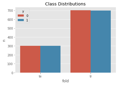
    temp = pd.concat([
        pd.DataFrame({'y': y_tr}).assign(fold='tr'),
        pd.DataFrame({'y': y_te}).assign(fold='te')
    ]).assign(n=1).groupby(['fold', 'y'])['n'].sum().to_frame().reset_index()
    fig, ax = plt.subplots()
    sns.barplot(x='fold', hue='y', y='n', data=temp, ax=ax)
    ax.set_title('Class Distributions')
    mlflow.log_figure(fig, 'fig/00-class-distributions.png')

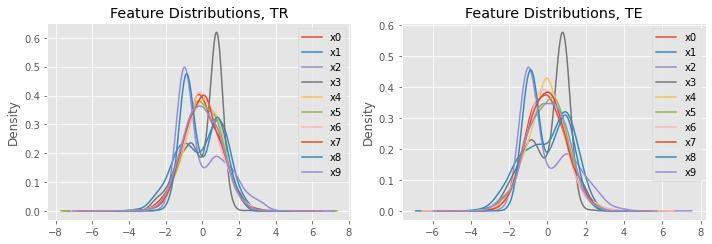
    fig, ax = plt.subplots(1, 2, figsize=(10, 3.5))
    X_tr.plot(kind='kde', ax=ax[0], title='Feature Distributions, TR')
    X_te.plot(kind='kde', ax=ax[1], title='Feature Distributions, TE')
    plt.tight_layout()
    mlflow.log_figure(fig, 'fig/01-feature-distributions.png')

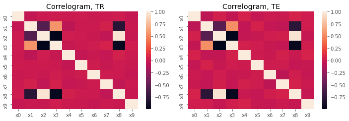
    fig, ax = plt.subplots(1, 2, figsize=(10, 3.5))
    sns.heatmap(X_tr.corr(), ax=ax[0])
    sns.heatmap(X_te.corr(), ax=ax[1])
    ax[0].set_title('Correlogram, TR')
    ax[1].set_title('Correlogram, TE')
    plt.tight_layout()
    mlflow.log_figure(fig, 'fig/02-correlograms.png')

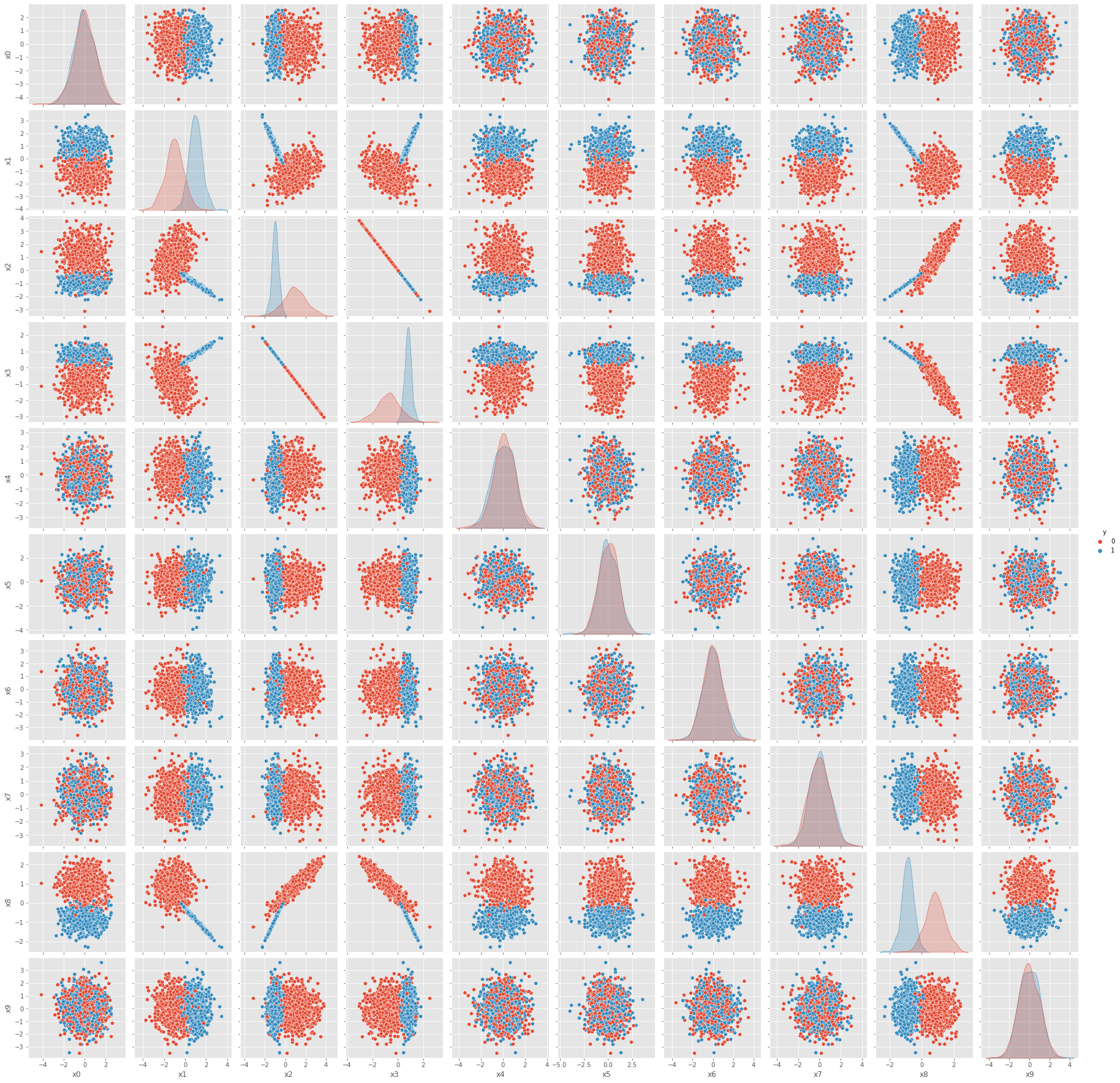
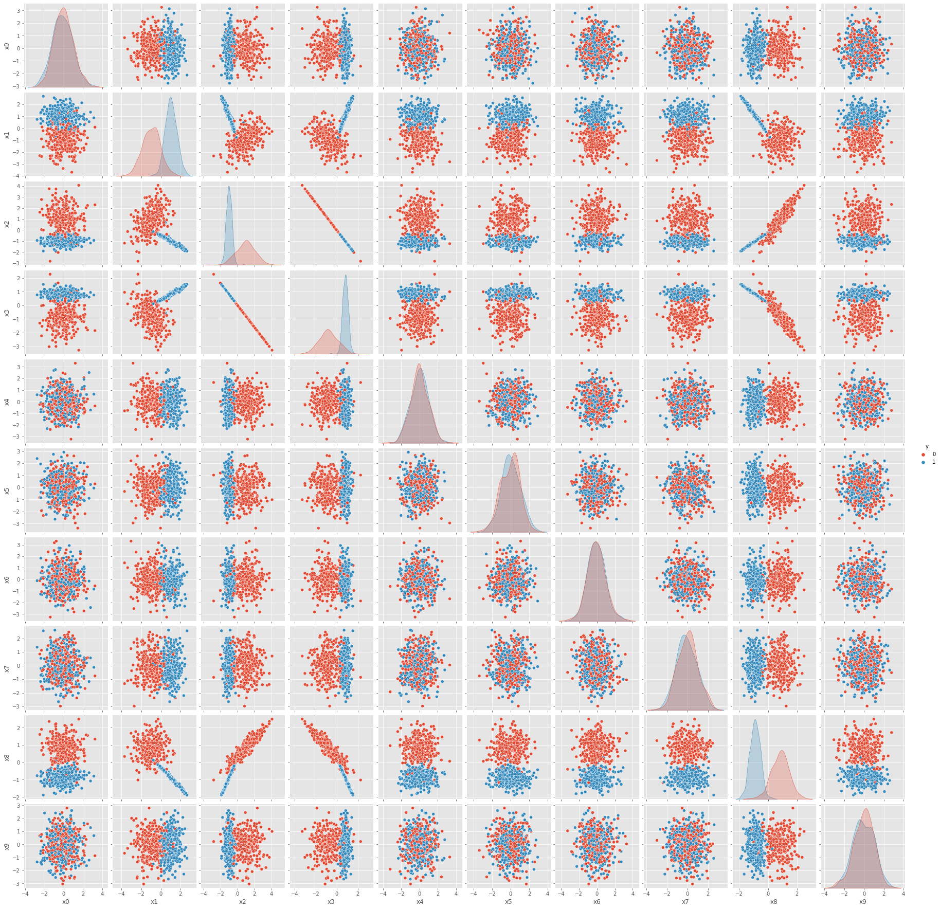
    fig = sns.pairplot(X_tr.assign(y=y_tr), hue='y').fig
    mlflow.log_figure(fig, 'fig/03-00-tr-pairplot.png')

    fig = sns.pairplot(X_te.assign(y=y_te), hue='y').fig
    mlflow.log_figure(fig, 'fig/03-01-te-pairplot.png')

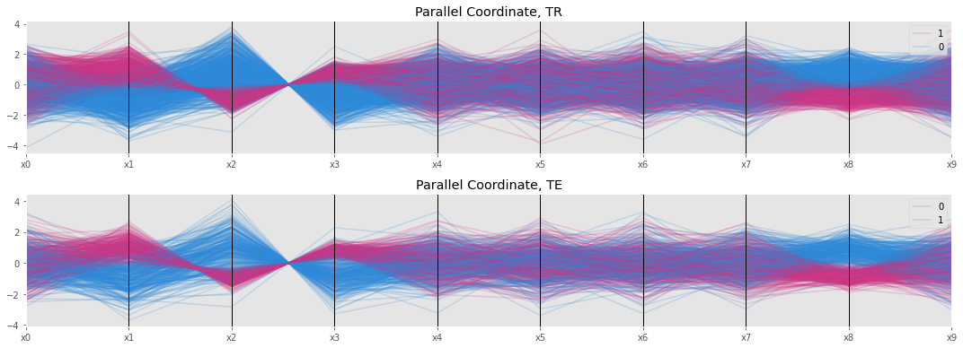
    fig, ax = plt.subplots(2, 1, figsize=(15, 5.5))
    pd.plotting.parallel_coordinates(X_tr.assign(y=y_tr), 'y', X_tr.columns, color=['#2e8ad8', '#cd3785'], sort_labels=True, axvlines=True, alpha=0.2, ax=ax[0])
    pd.plotting.parallel_coordinates(X_te.assign(y=y_te), 'y', X_tr.columns, color=['#2e8ad8', '#cd3785'], sort_labels=True, axvlines=True, alpha=0.2, ax=ax[1])
    ax[0].set_title('Parallel Coordinate, TR')
    ax[1].set_title('Parallel Coordinate, TE')
    plt.tight_layout()
    mlflow.log_figure(fig, 'fig/04-parallel-coordinate.png')

    run_id = mlflow.active_run().info.run_id
    print(f'run_id={run_id}')

Fitting 5 folds for each of 8 candidates, totalling 40 fits

2022/05/28 02:20:14 WARNING mlflow.utils.environment: Encountered an unexpected error while inferring pip requirements (model URI: /tmp/tmpsy1b58yj/model/model.pkl, flavor: sklearn), fall back to return ['scikit-learn==0.24.1', 'cloudpickle==1.6.0']. Set logging level to DEBUG to see the full traceback.

run_id=ae12b6f88a424d4783abb42b504f2bb7

Finally, we can load the model (using the run_id) and make predictions. Note how we persisted/logged the model using the sklearn flavor and also depersisted/loaded the model using the sklearn flavor again.

loaded_model = mlflow.sklearn.load_model(f'runs:/{run_id}/model')
loaded_model.predict_proba(X_tr)

array([[0.62361146, 0.37638854],
       [0.93569093, 0.06430907],
       [0.16239568, 0.83760432],
       ...,
       [0.0796527 , 0.9203473 ],
       [0.90753055, 0.09246945],
       [0.0532899 , 0.9467101 ]])

We can also spawn hundreds of independent training jobs with different hyperparameters (not using scikit’s grid search) and log each of them to MLflow.

path_tr = './_temp/tr.csv'
path_te = './_temp/te.csv'

X_tr.assign(y=y_tr).to_csv(path_tr, index=False)
X_te.assign(y=y_te).to_csv(path_te, index=False)

from joblib import Parallel, delayed

def do_learn(penalty, C, path_tr, path_te, tracking_uri='http://localhost:5001', experiment_name='test2'):
    def get_Xy(path):
        df = pd.read_csv(path)
        y_col = 'y'
        X_cols = [c for c in df.columns if c != y_col]

        X, y = df[X_cols], df[y_col]
        return X, y

    X_tr, y_tr = get_Xy(path_tr)
    X_te, y_te = get_Xy(path_te)

    model_params = {
        'solver': 'saga',
        'penalty': penalty,
        'C': C,
        'random_state': 37,
        'max_iter': 1_000
    }
    model = LogisticRegression(**model_params)

    if not mlflow.get_experiment_by_name(experiment_name):
        try:
            mlflow.create_experiment(experiment_name)
        except MlflowException as ex:
            print(f'{ex}')

    mlflow.set_tracking_uri(tracking_uri)
    mlflow.set_experiment(experiment_name)

    with mlflow.start_run() as run:
        model.fit(X_tr, y_tr)

        signature = infer_signature(X_tr, model.predict_proba(X_tr))
        mlflow.sklearn.log_model(model, 'model', signature=signature)
        mlflow.log_params(model_params)

        perf_metrics = get_performances(X_tr, y_tr, X_te, y_te, model)
        mlflow.log_metrics(perf_metrics)

        run_id = mlflow.active_run().info.run_id

    return run_id


size = 100
C = np.random.uniform(size=size)
P = np.random.uniform(size=size)
P = np.select([P < 0.5, P >= 0.5], ['l1', 'l2'])

run_ids = Parallel(n_jobs=-1)(delayed(do_learn)(p, c, path_tr, path_te) for p, c in zip(P, C))
print(run_ids)

['4b44a825df3a4a479a413fa5969db73d', '3cf7ab9496c243bf99f7159e3570118a', '1953685bd99e4c6ea7c9ccb054eee7cd', '9f84a08095b04136bd41ec43a36c038e', '5c5e69606bfc4a17ad17951d9e71e699', 'cc82e30810864e3db167cd993a9a93a5', '94a947fd86184fa8af1d02a7bc927065', '514c43c415a84637b64e7e0e852831b7', '15a9d5de992140c68d59f76f3e960f37', '9727bba9d8f248578bd13c493217e17f', '86b33b2bdd274227902ae59194aa3247', 'e7130921455640388278f92ddf599a84', '3e3492151163469aa1448fa57109db1b', '48d997b5d3674708ab5cb66bce21f767', '0c6a5f1ec98c4064bae68a4037680434', '78ea7dbfff124762b19796527df7d3ea', 'c412f93eeeb74aa5881e122b44e5f066', '623bb2a26dd744cd8b9c06af959d0e68', '011555648e6e4349bfb0b56c605b769d', 'c74c8daebbeb4062b9c561e59dac7eda', '40dae8a8fb9a495e924e48b0c5cb1117', 'f56529fef394418ca7888d5e268783d3', '2edeeb59f35f40e9aec6e66d3abe04c9', '78b6afca2c6d4497a18b92cb4422c4bd', '1931d4963b6341d6b995fc245ff3d42b', 'a93c2f7173f94b549913b7d4f2ed17de', 'a5b84397b3f34e8bab6cce66f171df83', '9881e992ba754310a4c048a5fd0175c4', '686be437b66c48d19e7e8160074e00eb', 'c038b25c59ee43339a515f541395547d', '8d7cae8317994c2a9406bb030968dc9d', 'f7882052620041f1ababcc60b26c98c3', '61d45b4eb6e840a594875707d0898971', '69f50a246c244d74ad5cf6b85fe483f3', '0eadfd2c706540f380b38f249db02589', 'cb5ab1b6472d401b91c397146508ecf3', '24e4a94e1800493d83a278c6dcf58886', 'a8cc5ff4f0f94746be7b180021debcfe', 'ec501330bff24e03887c6625b9e4230d', '73d06fe293794a44a7b6d915bc22d3da', 'f26a62b764f347f1a6969c3ce6ee0a2b', 'abe276323a4d466887696b946ded3db5', '5162825bd3a7426eb42b51d01fb35e70', '7b6dfb12feb84c929c76690694d64d56', '0cffadeb99044a33a3422bd73a046304', '1430eb8474514a5fb226f81739104e3c', '51d24c85d9934988b555794e83280d1d', '0f95d47b188f4a25b55e82a59187fa9c', '9a021acae1284677974e1b26ef35a21c', '8ee617aa9faa40ee92eeb575f0f01bc4', '27e191d655d24baa9533e2dc1a563561', 'dd5491d0010a4d9aa4d3ff4faddc1f33', 'afba4863360143a1841725a5e265aa6b', '8c750046d3f146adbc2370eba35afa64', '863ea7e694304610a2e2c98128bf2da8', 'de18890f47f246be80ee5b04767a2cfe', '569c3f719844453f831acf3b8626ac12', '59683d14ac9b439ebc411f681c2e9a67', '51573df0fb9a47ecb4c46e9bc9728902', 'fd34a5b4e7314611884e5b7677b79569', '230c156caa004a34b3f65793ad8c093e', '70e1020e91dd48b98e70a4dd9ac6185e', 'fccba53974a24eecbc2fd18438fdf551', '95c780fdb2a7406a837d0fc57634927a', 'c918e6b274a2420196765289ce4f9cec', '98d2124c64db46bc9717fb0d64afa602', 'c19f8545d8564975bdec4654a5dc1c11', '22ba3c251f724ca59a0a7ddb04c88479', 'd3f6924c0f5f410dbbb4baa3dd2de298', '4b751b0557a74103baa51f4d0bd8ec76', '2f392a19b07b402692b98f5ee9a39107', 'efef9b825e1746a883c0ae92b977db77', '2a898c0f68364e789375890ad54f6611', '2949a480136a4205899baad415cae1af', '7b063f4bcb874fd7b8a83e594ac52127', 'd9ba46081def41bc82a3478d299ceb10', 'b8b134632bbc476c97efc18376b9818e', '0c898f4713ee4a70a824d556e49c68ba', '8ad093566b474c35b6653e130278fe14', '85aa3749f0a948c8a90c11d86fec0987', 'a2f215e457ac4762a070b1843d39882e', 'fa059ec7116e482a854a0bdbd12c5692', 'a287b292fc67475290b525d8e9ff20e3', '61e43d866e7542a78bd9d2444c4a89b1', '806b00d52b634a139c51ab7362c9c7c4', '76aba9fbd1d64e63910dfcc881c79d77', '7df4d76ab7ab4b49a1efebc4ba0eb581', '64e5db3322a547b2976d2874e2e95ec8', '36fa6b0977394e44b34d2d8bf650dd0a', '4e5e4ffba90247ff9f215f274db80bda', '69546ea7050d4a53bde498b1725aaac6', '798fbb91e095417fad2ed86a5d2beea2', '21c23f487197471ea7826c0fe2df8d22', '553091345c5f4022b6603e0ca41b0f8d', 'ce67378fa92947ddbd395619fe5315de', 'bae016b49ade45bfb0ded139db5f8ba9', '1f9c2e5f46984272aa8fecf6800ae1c4', '1e033341ce5246618c36c9662be54b51', '71b1699097c94d5586455a83494afbb6', '1ef399eba3634096b981ca46f2c3e4f6']

We can then collect the parameters and performances and do modeling to see how the parameters impact the performances.

• The regularization term C seems to be very important in average precision score and AUC.

• The regularization approach l1=1 and l2=2 seems to be more important in F1 score.

O = pd.DataFrame(map(lambda i: mlflow.get_run(i).data.metrics, run_ids))

I = pd.DataFrame(map(lambda i: mlflow.get_run(i).data.params, run_ids)) \
    .assign(penalty=lambda d: d['penalty'].apply(lambda v: 1 if v == 'l1' else 2)) \
    [['penalty', 'C']]

from sklearn.ensemble import RandomForestRegressor

pd.Series(RandomForestRegressor().fit(I, O['aps_te']).feature_importances_, index=I.columns)

penalty    0.265576
C          0.734424
dtype: float64

pd.Series(RandomForestRegressor().fit(I, O['auc_te']).feature_importances_, index=I.columns)

penalty    0.332347
C          0.667653
dtype: float64

pd.Series(RandomForestRegressor().fit(I, O['f1_te']).feature_importances_, index=I.columns)

penalty    0.698958
C          0.301042
dtype: float64