1. Pandas
pandas stands for Python Data Analysis Library. Two of the main data structures in pandas are Series and DataFrame. The series data structure is a glorified list with batteries included, and the dataframe is a glorified table with extra, extra batteries included. You get a lot of additional and handy features by using these data structures to store and represent your data as lists or tables.
1.1. Pandas Series
The easiest way to understand a Series is to simply create one. At the data level, a series is simply just a list of data.
[1]:
import pandas as pd

s = pd.Series([1, 2, 3, 4])
s
[1]:
0    1
1    2
2    3
3    4
dtype: int64
With every element in the list is a corresponding index. The index may not seem important at first glance, but it is very important later when you need to filter or slice the series. If you do not specify the index for each element, a sequential and numeric one is created automatically (starting from zero). Here is how you can create a series with the index specified.
[2]:
s = pd.Series([1, 2, 3, 4], index=[10, 11, 12, 13])
s
[2]:
10    1
11    2
12    3
13    4
dtype: int64
The index can also be string type.
[3]:
s = pd.Series([1, 2, 3, 4], index=['a', 'b', 'c', 'd'])
s
[3]:
a    1
b    2
c    3
d    4
dtype: int64
You can access the index and values of a series individually.
[4]:
s.index
[4]:
Index(['a', 'b', 'c', 'd'], dtype='object')
[5]:
s.values
[5]:
array([1, 2, 3, 4])
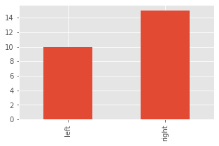
Why would you ever want string values for an index? Let’s say we have a count of left and right handedness in a room. We can represent this data as a series.
[6]:
s = pd.Series([10, 15], index=['left', 'right'])
s
[6]:
left     10
right    15
dtype: int64
And then, we can magically plot the bar chart showing the counts of left and right handedness in the room.
[7]:
import matplotlib.pyplot as plt
plt.style.use('ggplot')

fig, ax = plt.subplots(figsize=(5, 3))
_ = s.plot(kind='bar', ax=ax)
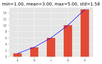
1.1.1. Functions
There are just too many useful functions attached to a series. Here’s a few that are interesting.
[8]:
s = pd.Series([1, 2, 3, 4, 5], index=['a', 'b', 'c', 'd', 'e'])
_mean = s.mean()
_min = s.min()
_max = s.max()
_std = s.std()

fig, ax = plt.subplots(figsize=(5, 3))
_ = s.cumsum().plot(kind='bar', ax=ax)
_ = s.cumsum().plot(kind='line', ax=ax, color='blue')
_ = ax.set_title(f'min={_min:.2f}, mean={_mean:.2f}, max={_max:.2f}, std={_std:.2f}')
The value_counts() function can quickly give you the frequencies of unique values.
[9]:
s = pd.Series([1, 1, 2, 2, 2, 3, 3, 4, 4, 4, 4])
s.value_counts()
[9]:
4    4
2    3
3    2
1    2
dtype: int64
1.1.2. Filtering
Filtering is important. Let’s see how to filter based on values.
[10]:
s = pd.Series([1, 2, 3, 4])
s1 = s[s > 2]
s1
[10]:
2    3
3    4
dtype: int64
How do we filter based on index?
[11]:
s2 = s[s.index < 2]
s2
[11]:
0    1
1    2
dtype: int64
[12]:
s2 = s[s.index.isin([0, 1])]
s2
[12]:
0    1
1    2
dtype: int64
1.1.3. Iteration
Iteration of the index and values of a series is accomplished with zip.
[13]:
s = pd.Series([1, 2, 3, 4, 5], index=['a', 'b', 'c', 'd', 'e'])
for i, v in zip(s.index, s.values):
    print(f'{i}: {v}')
a: 1
b: 2
c: 3
d: 4
e: 5
1.1.4. To dataframe
We will talk about Pandas dataframes next, but for now, it’s quite easy to convert a series to a dataframe using .to_frame(). Note that we have to supply the name so that the column name is meaningful.
[14]:
s = pd.Series([1, 2, 3, 4, 5], index=['a', 'b', 'c', 'd', 'e'], name='number')
s
[14]:
a    1
b    2
c    3
d    4
e    5
Name: number, dtype: int64
[15]:
s.to_frame()
[15]:
| number | |
|---|---|
| a | 1 |
| b | 2 |
| c | 3 |
| d | 4 |
| e | 5 |
1.2. Pandas Dataframes
Dataframes are the most powerful data structure in pandas. As a start, it’s helpful to simply think of a dataframe as a table. Below, we create a dataframe from a list of tuples, where each tuple is a pair of numbers. Notice how the columns are not specified and so they default to 0 and 1, and the index is not specified so a numeric, sequential one is created.
[16]:
df = pd.DataFrame([(1, 2), (3, 4), (5, 6)])
df
[16]:
| 0 | 1 | |
|---|---|---|
| 0 | 1 | 2 |
| 1 | 3 | 4 |
| 2 | 5 | 6 |
If we wanted to specify the column names, supply a list of column names.
[17]:
df = pd.DataFrame([(1, 2), (3, 4), (5, 6)], columns=['x', 'y'])
df
[17]:
| x | y | |
|---|---|---|
| 0 | 1 | 2 |
| 1 | 3 | 4 |
| 2 | 5 | 6 |
If we need to specify the index, supply a list of index for each row.
[18]:
df = pd.DataFrame([(1, 2), (3, 4), (5, 6)], columns=['x', 'y'], index=['a', 'b', 'c'])
df
[18]:
| x | y | |
|---|---|---|
| a | 1 | 2 |
| b | 3 | 4 |
| c | 5 | 6 |
There’s other ways to create a dataframe. Let’s use a list of dictionaries. Notice how we do not need to supply a list of column names?
[19]:
df = pd.DataFrame([
    {'x': 1, 'y': 2},
    {'x': 3, 'y': 4},
    {'x': 5, 'y': 6}
], index=['a', 'b', 'c'])
df
[19]:
| x | y | |
|---|---|---|
| a | 1 | 2 |
| b | 3 | 4 |
| c | 5 | 6 |
Above, we used a list of dictionaries, below, we use a dictionary of lists.
[20]:
df = pd.DataFrame({
    'x': [1, 3, 4],
    'y': [2, 4, 5]
}, index=['a', 'b', 'c'])
df
[20]:
| x | y | |
|---|---|---|
| a | 1 | 2 |
| b | 3 | 4 |
| c | 4 | 5 |
1.2.1. Properties
There’s a lot of neat and useful properties and functions attached to a dataframe. The dtypes property gives you the data types of your fields.
[21]:
df.dtypes
[21]:
x    int64
y    int64
dtype: object
You can set the type of your data when you create a data frame by supplying the dtype value.
[22]:
df = pd.DataFrame({
    'x': [1, 3, 4],
    'y': [2, 4, 5]
}, index=['a', 'b', 'c'], dtype='int32')
df.dtypes
[22]:
x    int32
y    int32
dtype: object
Look at what happens when you have missing values and do not specify the type. The y column is now of type float64.
[23]:
df = pd.DataFrame({
    'x': [1, 3, 4],
    'y': [2, 4, None]
}, index=['a', 'b', 'c'])
df.dtypes
[23]:
x      int64
y    float64
dtype: object
Look at what happens when you have missing values and attempt to specify the type. The y column is now of type object.
[24]:
df = pd.DataFrame({
    'x': pd.Series([1, 3, 4], dtype='Int32'),
    'y': pd.Series([2, 4, None], dtype='Int32')
}, index=['a', 'b', 'c'])
df.dtypes
[24]:
x     int32
y    object
dtype: object
If you need to know the dimensions of your dataframe, use the shape property.
[25]:
df = pd.DataFrame({
    'x': [1, 3, 4],
    'y': [2, 4, 5]
}, index=['a', 'b', 'c'])

df.shape
[25]:
(3, 2)
You can turn your dataframe into a numpy array using values.
[26]:
df.values
[26]:
array([[1, 2],
       [3, 4],
       [4, 5]])
1.2.2. Columns or fields
You can access each column by bracket [] or dot notation .. To access a column by name, specify the column name inside the brackets.
[27]:
df['x']
[27]:
a    1
b    3
c    4
Name: x, dtype: int64
[28]:
df['y']
[28]:
a    2
b    4
c    5
Name: y, dtype: int64
Multiple columns may be selecting by passing a list of column names.
[29]:
df[['x', 'y']]
[29]:
| x | y | |
|---|---|---|
| a | 1 | 2 |
| b | 3 | 4 |
| c | 4 | 5 |
To access the columns by dot notation, do the following. Be careful when accessing columns/fields using dot notation; if you have a field that is named the same as a function attached to the dataframe (e.g. mean), the function has precedence over the field (e.g. df['mean'] is preferred over df.mean).
[30]:
df.x
[30]:
a    1
b    3
c    4
Name: x, dtype: int64
[31]:
df.y
[31]:
a    2
b    4
c    5
Name: y, dtype: int64
Note that accessing a column will return that column as a series, and the usual series properties and functions may be applied.
[32]:
df.x.sum()
[32]:
8
[33]:
df.x.mean()
[33]:
2.6666666666666665
[34]:
df.x.std()
[34]:
1.5275252316519465
[35]:
df.x.min()
[35]:
1
[36]:
df.x.max()
[36]:
4
1.2.3. Rows or records
To access the rows or records, use iloc and specify the numeric location value or loc and specify the index value. Below, .iloc[0] refers to the first record.
[37]:
df.iloc[0]
[37]:
x    1
y    2
Name: a, dtype: int64
Below, .loc['a'] refers to the row corresponding to the a index value.
[38]:
df.loc['a']
[38]:
x    1
y    2
Name: a, dtype: int64
Multiple rows may be selected by numeric index through slicing.
[39]:
df.iloc[0:2]
[39]:
| x | y | |
|---|---|---|
| a | 1 | 2 |
| b | 3 | 4 |
[40]:
df.iloc[2:3]
[40]:
| x | y | |
|---|---|---|
| c | 4 | 5 |
Accessing rows/records using loc or iloc typically returns another dataframe (as opposed to bracket and dot notations with columns, which returns a series).
1.2.4. Methods
Use describe() to get summary statistics over your fields.
[41]:
df.describe()
[41]:
| x | y | |
|---|---|---|
| count | 3.000000 | 3.000000 |
| mean | 2.666667 | 3.666667 |
| std | 1.527525 | 1.527525 |
| min | 1.000000 | 2.000000 |
| 25% | 2.000000 | 3.000000 |
| 50% | 3.000000 | 4.000000 |
| 75% | 3.500000 | 4.500000 |
| max | 4.000000 | 5.000000 |
The info() method gives other types of field profiling information.
[42]:
df.info()
<class 'pandas.core.frame.DataFrame'>
Index: 3 entries, a to c
Data columns (total 2 columns):
 #   Column  Non-Null Count  Dtype
---  ------  --------------  -----
 0   x       3 non-null      int64
 1   y       3 non-null      int64
dtypes: int64(2)
memory usage: 152.0+ bytes
The cummulative sum is retrieved by calling cumsum().
[43]:
df.cumsum()
[43]:
| x | y | |
|---|---|---|
| a | 1 | 2 |
| b | 4 | 6 |
| c | 8 | 11 |
You can mathematically operate on a dataframe. Below, we turn the integer values into percentages.
[44]:
df / df.sum()
[44]:
| x | y | |
|---|---|---|
| a | 0.125 | 0.181818 |
| b | 0.375 | 0.363636 |
| c | 0.500 | 0.454545 |
Transposing is easy.
[45]:
df.transpose()
[45]:
| a | b | c | |
|---|---|---|---|
| x | 1 | 3 | 4 |
| y | 2 | 4 | 5 |
You can also transpose a dataframe as follows.
[46]:
df.T
[46]:
| a | b | c | |
|---|---|---|---|
| x | 1 | 3 | 4 |
| y | 2 | 4 | 5 |
1.2.5. Conversion
There’s quite a few different ways to convert fields.
[47]:
df = pd.DataFrame({
    'x': [1.0, 2.0, 3.0],
    'y': ['2021-12-01', '2021-12-02', '2021-12-03'],
    'z': ['10', '20', '30']
})

df
[47]:
| x | y | z | |
|---|---|---|---|
| 0 | 1.0 | 2021-12-01 | 10 |
| 1 | 2.0 | 2021-12-02 | 20 |
| 2 | 3.0 | 2021-12-03 | 30 |
Use pd.to_datetime() to convert str to datetime64[ns].
[48]:
pd.to_datetime(df.y)
[48]:
0   2021-12-01
1   2021-12-02
2   2021-12-03
Name: y, dtype: datetime64[ns]
[49]:
pd.to_datetime(df.y, format='%Y-%m-%d')
[49]:
0   2021-12-01
1   2021-12-02
2   2021-12-03
Name: y, dtype: datetime64[ns]
The astype() function can also be used to convert data types.
[50]:
df['y'].astype('datetime64[ns]')
[50]:
0   2021-12-01
1   2021-12-02
2   2021-12-03
Name: y, dtype: datetime64[ns]
[51]:
df['x'].astype('int')
[51]:
0    1
1    2
2    3
Name: x, dtype: int64
[52]:
df['z'].astype('int')
[52]:
0    10
1    20
2    30
Name: z, dtype: int64
1.2.6. Joining and concatenating
Dataframes can be joined. The easiest way is to join two dataframes based on index values. This stacks up the dataframes horizontally or the wide way.
[53]:
df1 = pd.DataFrame({
    'x': [1, 3, 4],
    'y': [2, 4, 5]
}, index=['a', 'b', 'c'])

df2 = pd.DataFrame({
    'v': [6, 7, 8],
    'w': [9, 10, 11]
}, index=['a', 'b', 'c'])

df1.join(df2)
[53]:
| x | y | v | w | |
|---|---|---|---|---|
| a | 1 | 2 | 6 | 9 |
| b | 3 | 4 | 7 | 10 |
| c | 4 | 5 | 8 | 11 |
If the field you want to join on is not in the index, you can set the index set_index() to the field you want to join on at join time.
[54]:
df1 = pd.DataFrame({
    'id': ['a', 'b', 'c'],
    'x': [1, 3, 4],
    'y': [2, 4, 5]
})

df2 = pd.DataFrame({
    'id': ['a', 'b', 'c'],
    'v': [6, 7, 8],
    'w': [9, 10, 11]
})

df1.set_index('id') \
    .join(df2.set_index('id'))
[54]:
| x | y | v | w | |
|---|---|---|---|---|
| id | ||||
| a | 1 | 2 | 6 | 9 |
| b | 3 | 4 | 7 | 10 |
| c | 4 | 5 | 8 | 11 |
If you want the id colum back into the dataframe, then call reset_index() after joining.
[55]:
df1.set_index('id') \
    .join(df2.set_index('id')) \
    .reset_index()
[55]:
| id | x | y | v | w | |
|---|---|---|---|---|---|
| 0 | a | 1 | 2 | 6 | 9 |
| 1 | b | 3 | 4 | 7 | 10 |
| 2 | c | 4 | 5 | 8 | 11 |
Dataframes can also be concatenated vertically or the long way.
[56]:
df1 = pd.DataFrame({
    'x': [1, 3, 4],
    'y': [2, 4, 5]
}, index=['a', 'b', 'c'])

df2 = pd.DataFrame({
    'x': [6, 7, 8],
    'y': [9, 10, 11]
}, index=['d', 'e', 'f'])

pd.concat([df1, df2])
[56]:
| x | y | |
|---|---|---|
| a | 1 | 2 |
| b | 3 | 4 |
| c | 4 | 5 |
| d | 6 | 9 |
| e | 7 | 10 |
| f | 8 | 11 |
1.2.7. Multiple indexes
Indexes plays a very important role in organizing your data in a dataframe. For the most part, we have shown a single index on a dataframe. But a dataframe can have a multiple indices using MultiIndex. Below, we create a fictitious set of data of handedness and sports by gender.
[57]:
row_index = pd.MultiIndex.from_tuples([
    ('left', 'soccer'),
    ('left', 'baseball'),
    ('right', 'soccer'),
    ('right', 'baseball')])
data = {
    'male': [5, 10, 15, 20],
    'female': [6, 11, 20, 25]
}
pd.DataFrame(data, index=row_index)
[57]:
| male | female | ||
|---|---|---|---|
| left | soccer | 5 | 6 |
| baseball | 10 | 11 | |
| right | soccer | 15 | 20 |
| baseball | 20 | 25 |
The column index can also have multiple indexes.
[58]:
row_index = pd.MultiIndex.from_tuples([
    ('left', 'soccer'),
    ('left', 'baseball'),
    ('right', 'soccer'),
    ('right', 'baseball')])

col_index = pd.MultiIndex.from_tuples([
    ('amateur', 'male'),
    ('amateur', 'female'),
    ('pro', 'male'),
    ('pro', 'female')
])

data = [
    [5, 10, 15, 20],
    [6, 11, 20, 25],
    [10, 11, 25, 30],
    [15, 17, 30, 35]
]

df = pd.DataFrame(data, index=row_index, columns=col_index)
df
[58]:
| amateur | pro | ||||
|---|---|---|---|---|---|
| male | female | male | female | ||
| left | soccer | 5 | 10 | 15 | 20 |
| baseball | 6 | 11 | 20 | 25 | |
| right | soccer | 10 | 11 | 25 | 30 |
| baseball | 15 | 17 | 30 | 35 | |
1.2.8. Filtering rows
Let’s see how filtering for records in a dataframe works. One filtering approach is by index.
[59]:
df = pd.DataFrame({
    'x': [1, 3, 4],
    'y': [2, 4, 5]
}, index=['a', 'b', 'c'])


df[df.x >= 3]
[59]:
| x | y | |
|---|---|---|
| b | 3 | 4 |
| c | 4 | 5 |
We can filter by index using boolean logic with and (&) or or (|). Notice how we have to use parentheses around the comparisons?
[60]:
df[(df.x >= 3) & (df.y > 4)]
[60]:
| x | y | |
|---|---|---|
| c | 4 | 5 |
[61]:
df[(df.x >= 3) | (df.y > 4)]
[61]:
| x | y | |
|---|---|---|
| b | 3 | 4 |
| c | 4 | 5 |
If you are familiar with Structured Query Language SQL, you can filter using the query() method specifying the conditions as in a SQL where clause.
[62]:
df.query('x >= 3 and y > 4')
[62]:
| x | y | |
|---|---|---|
| c | 4 | 5 |
[63]:
df.query('x >= 3 or y > 4')
[63]:
| x | y | |
|---|---|---|
| b | 3 | 4 |
| c | 4 | 5 |
You can also use numpy to filter rows.
[64]:
import numpy as np

df[np.logical_and(df.x >= 3, df.y > 4)]
[64]:
| x | y | |
|---|---|---|
| c | 4 | 5 |
[65]:
df[np.logical_or(df.x >= 3, df.y > 4)]
[65]:
| x | y | |
|---|---|---|
| b | 3 | 4 |
| c | 4 | 5 |
[66]:
df[np.logical_not(df.x == 3)]
[66]:
| x | y | |
|---|---|---|
| a | 1 | 2 |
| c | 4 | 5 |
What about filtering date fields?
[67]:
df = pd.DataFrame({
    'x': [i for i in range(1, 32)],
    'y': pd.to_datetime([f'2021-12-{i:02}' for i in range(1, 32)])
})

df.head()
[67]:
| x | y | |
|---|---|---|
| 0 | 1 | 2021-12-01 |
| 1 | 2 | 2021-12-02 |
| 2 | 3 | 2021-12-03 |
| 3 | 4 | 2021-12-04 |
| 4 | 5 | 2021-12-05 |
[68]:
df.query('y > "2021-12-25"')
[68]:
| x | y | |
|---|---|---|
| 25 | 26 | 2021-12-26 |
| 26 | 27 | 2021-12-27 |
| 27 | 28 | 2021-12-28 |
| 28 | 29 | 2021-12-29 |
| 29 | 30 | 2021-12-30 |
| 30 | 31 | 2021-12-31 |
[69]:
df[df.y > '2021-12-25']
[69]:
| x | y | |
|---|---|---|
| 25 | 26 | 2021-12-26 |
| 26 | 27 | 2021-12-27 |
| 27 | 28 | 2021-12-28 |
| 28 | 29 | 2021-12-29 |
| 29 | 30 | 2021-12-30 |
| 30 | 31 | 2021-12-31 |
[70]:
df.query('"2021-12-20" < y < "2021-12-25"')
[70]:
| x | y | |
|---|---|---|
| 20 | 21 | 2021-12-21 |
| 21 | 22 | 2021-12-22 |
| 22 | 23 | 2021-12-23 |
| 23 | 24 | 2021-12-24 |
[71]:
df[('2021-12-20' < df.y) & (df.y < '2021-12-25')]
[71]:
| x | y | |
|---|---|---|
| 20 | 21 | 2021-12-21 |
| 21 | 22 | 2021-12-22 |
| 22 | 23 | 2021-12-23 |
| 23 | 24 | 2021-12-24 |
What about filtering against a multi-index?
[72]:
row_index = pd.MultiIndex.from_tuples([
    ('left', 'soccer'),
    ('left', 'baseball'),
    ('right', 'soccer'),
    ('right', 'baseball')])

col_index = pd.MultiIndex.from_tuples([
    ('amateur', 'male'),
    ('amateur', 'female'),
    ('pro', 'male'),
    ('pro', 'female')
])

data = [
    [5, 10, 15, 20],
    [6, 11, 20, 25],
    [10, 11, 25, 30],
    [15, 17, 30, 35]
]

df = pd.DataFrame(data, index=row_index, columns=col_index)
df
[72]:
| amateur | pro | ||||
|---|---|---|---|---|---|
| male | female | male | female | ||
| left | soccer | 5 | 10 | 15 | 20 |
| baseball | 6 | 11 | 20 | 25 | |
| right | soccer | 10 | 11 | 25 | 30 |
| baseball | 15 | 17 | 30 | 35 | |
[73]:
df[df.index.isin(['left'], level=0)]
[73]:
| amateur | pro | ||||
|---|---|---|---|---|---|
| male | female | male | female | ||
| left | soccer | 5 | 10 | 15 | 20 |
| baseball | 6 | 11 | 20 | 25 | |
[74]:
df[df.index.isin(['right'], level=0)]
[74]:
| amateur | pro | ||||
|---|---|---|---|---|---|
| male | female | male | female | ||
| right | soccer | 10 | 11 | 25 | 30 |
| baseball | 15 | 17 | 30 | 35 | |
[75]:
df[df.index.isin(['soccer'], level=1)]
[75]:
| amateur | pro | ||||
|---|---|---|---|---|---|
| male | female | male | female | ||
| left | soccer | 5 | 10 | 15 | 20 |
| right | soccer | 10 | 11 | 25 | 30 |
[76]:
df[df.index.isin(['baseball'], level=1)]
[76]:
| amateur | pro | ||||
|---|---|---|---|---|---|
| male | female | male | female | ||
| left | baseball | 6 | 11 | 20 | 25 |
| right | baseball | 15 | 17 | 30 | 35 |
1.2.9. Filtering columns
What about subsetting or slicing multi-index columns?
[77]:
df.loc[:, df.columns.get_level_values(0).isin(['amateur'])]
[77]:
| amateur | |||
|---|---|---|---|
| male | female | ||
| left | soccer | 5 | 10 |
| baseball | 6 | 11 | |
| right | soccer | 10 | 11 |
| baseball | 15 | 17 | |
[78]:
df.loc[:, df.columns.get_level_values(0).isin(['pro'])]
[78]:
| pro | |||
|---|---|---|---|
| male | female | ||
| left | soccer | 15 | 20 |
| baseball | 20 | 25 | |
| right | soccer | 25 | 30 |
| baseball | 30 | 35 | |
[79]:
df.loc[:, df.columns.get_level_values(1).isin(['male'])]
[79]:
| amateur | pro | ||
|---|---|---|---|
| male | male | ||
| left | soccer | 5 | 15 |
| baseball | 6 | 20 | |
| right | soccer | 10 | 25 |
| baseball | 15 | 30 |
[80]:
df.loc[:, df.columns.get_level_values(1).isin(['female'])]
[80]:
| amateur | pro | ||
|---|---|---|---|
| female | female | ||
| left | soccer | 10 | 20 |
| baseball | 11 | 25 | |
| right | soccer | 11 | 30 |
| baseball | 17 | 35 |
1.2.10. Iteration
How do we iterate over a dataframe? Use the iterrows() function.
[81]:
df = pd.DataFrame({
    'x': [1, 3, 4],
    'y': [2, 4, 5]
}, index=['a', 'b', 'c'])

for _index, row in df.iterrows():
    s = {c: row[c] for c in df.columns}
    print(f'{_index}: {s}')
a: {'x': 1, 'y': 2}
b: {'x': 3, 'y': 4}
c: {'x': 4, 'y': 5}
1.2.11. Transformation by row
What if we want to create a new column based on the whole row? Use the apply method on the dataframe and specify the axis to be 1 for column.
[82]:
df = pd.DataFrame({
    'x': [1, 3, 4],
    'y': [2, 4, 5]
}, index=['a', 'b', 'c'])

df['z'] = df.apply(lambda r: r.x + r.y, axis=1)
df
[82]:
| x | y | z | |
|---|---|---|---|
| a | 1 | 2 | 3 |
| b | 3 | 4 | 7 |
| c | 4 | 5 | 9 |
1.2.12. Transformation by column
What if we want to create a new column based on a column? Use the apply method on the column.
[83]:
df = pd.DataFrame({
    'x': [1, 3, 4],
    'y': [2, 4, 5]
}, index=['a', 'b', 'c'])

df['z'] = df.x.apply(lambda x: x**2)
df
[83]:
| x | y | z | |
|---|---|---|---|
| a | 1 | 2 | 1 |
| b | 3 | 4 | 9 |
| c | 4 | 5 | 16 |
1.2.13. Transformation of a dataframe
If you need to transform the dataframe as a whole, you should use the pipe() function which can be chained in a fluent way. Below, we have made up data on students; we have their handedness and overall numeric grade. We want to transform the encoding of handedness from 0 and 1 to left and right, respectively, and also numeric grade to letter grade. It will be fun to also transform the name to be properly cased and decomposed into its component parts (first name and last name).
[84]:
df = pd.DataFrame({
    'name': ['john doe', 'jack smith', 'jason demming', 'joe turing'],
    'handedness': [0, 1, 0, 1],
    'score': [0.95, 0.85, 0.75, 0.65]
})
df
[84]:
| name | handedness | score | |
|---|---|---|---|
| 0 | john doe | 0 | 0.95 |
| 1 | jack smith | 1 | 0.85 |
| 2 | jason demming | 0 | 0.75 |
| 3 | joe turing | 1 | 0.65 |
Take notice that each of these transformations return the dataframe. Otherwise, you will have None returned and chaining will break.
[85]:
def properly_case(df):
    df.name = df.name.apply(lambda n: n.title())
    return df

def decompose_name(df):
    df['first_name'] = df.name.apply(lambda n: n.split(' ')[0].strip())
    df['last_name'] = df.name.apply(lambda n: n.split(' ')[1].strip())
    return df

def reencode_handedness(df):
    df.handedness = df.handedness.apply(lambda h: 'left' if h == 0 else 'right')
    return df

def convert_letter_grade(df):
    def get_letter_grade(g):
        if g >= 0.90:
            return 'A'
        elif g >= 0.80:
            return 'B'
        elif g >= 0.70:
            return 'C'
        elif g >= 0.60:
            return 'D'
        else:
            return 'F'
    df['grade'] = df.score.apply(lambda s: get_letter_grade(s))
    return df

df = pd.DataFrame({
    'name': ['john doe', 'jack smith', 'jason demming', 'joe turing'],
    'handedness': [0, 1, 0, 1],
    'score': [0.95, 0.85, 0.75, 0.65]
})

df \
    .pipe(properly_case) \
    .pipe(decompose_name) \
    .pipe(reencode_handedness) \
    .pipe(convert_letter_grade)

df
[85]:
| name | handedness | score | first_name | last_name | grade | |
|---|---|---|---|---|---|---|
| 0 | John Doe | left | 0.95 | John | Doe | A |
| 1 | Jack Smith | right | 0.85 | Jack | Smith | B |
| 2 | Jason Demming | left | 0.75 | Jason | Demming | C |
| 3 | Joe Turing | right | 0.65 | Joe | Turing | D |
If you are piping a lot transformations, use the line continuation character \.
[86]:
df = pd.DataFrame({
    'name': ['john doe', 'jack smith', 'jason demming', 'joe turing'],
    'handedness': [0, 1, 0, 1],
    'score': [0.95, 0.85, 0.75, 0.65]
})

df = df.pipe(properly_case)\
        .pipe(decompose_name)\
        .pipe(reencode_handedness)\
        .pipe(convert_letter_grade)

df
[86]:
| name | handedness | score | first_name | last_name | grade | |
|---|---|---|---|---|---|---|
| 0 | John Doe | left | 0.95 | John | Doe | A |
| 1 | Jack Smith | right | 0.85 | Jack | Smith | B |
| 2 | Jason Demming | left | 0.75 | Jason | Demming | C |
| 3 | Joe Turing | right | 0.65 | Joe | Turing | D |
The line continuation character can become a nuisance, so wrap your chaining inside parentheses.
[87]:
df = pd.DataFrame({
    'name': ['john doe', 'jack smith', 'jason demming', 'joe turing'],
    'handedness': [0, 1, 0, 1],
    'score': [0.95, 0.85, 0.75, 0.65]
})

df = (df.pipe(properly_case)
        .pipe(decompose_name)
        .pipe(reencode_handedness)
        .pipe(convert_letter_grade))

df
[87]:
| name | handedness | score | first_name | last_name | grade | |
|---|---|---|---|---|---|---|
| 0 | John Doe | left | 0.95 | John | Doe | A |
| 1 | Jack Smith | right | 0.85 | Jack | Smith | B |
| 2 | Jason Demming | left | 0.75 | Jason | Demming | C |
| 3 | Joe Turing | right | 0.65 | Joe | Turing | D |
You can also use the assign() function to modify columns or create new ones. The difference between pipe() and assign() is that the former can create multiple columns per invocation and the latter is used to create one column per invocation.
[88]:
score2grade = lambda s: 'A' if s >= 0.9 else 'B' if s >= 0.8 else 'C' if s >= 0.7 else 'D' if s >= 0.6 else 'F'

pd.DataFrame({
    'name': ['john doe', 'jack smith', 'jason demming', 'joe turing'],
    'handedness': [0, 1, 0, 1],
    'score': [0.95, 0.85, 0.75, 0.65]
}).assign(
    name=lambda d: d['name'].apply(lambda n: n.title()),
    handedness=lambda d: d['handedness'].apply(lambda h: 'left' if h == 0 else 'right'),
    first_name=lambda d: d['name'].apply(lambda n: n.split(' ')[0]),
    last_name=lambda d: d['name'].apply(lambda n: n.split(' ')[1]),
    grade=lambda d: d['score'].apply(score2grade)
)
[88]:
| name | handedness | score | first_name | last_name | grade | |
|---|---|---|---|---|---|---|
| 0 | John Doe | left | 0.95 | John | Doe | A |
| 1 | Jack Smith | right | 0.85 | Jack | Smith | B |
| 2 | Jason Demming | left | 0.75 | Jason | Demming | C |
| 3 | Joe Turing | right | 0.65 | Joe | Turing | D |
The assign() function also takes in a dictionary where keys are strings (field names) and values are callable.
[89]:
pd.DataFrame({
    'name': ['john doe', 'jack smith', 'jason demming', 'joe turing'],
    'handedness': [0, 1, 0, 1],
    'spelling': [0.95, 0.85, 0.75, 0.65],
    'math': [0.65, 0.75, 0.85, 0.95]
}).assign(**{
    'spelling': lambda d: d['spelling'].apply(score2grade),
    'math': lambda d: d['math'].apply(score2grade)
})
[89]:
| name | handedness | spelling | math | |
|---|---|---|---|---|
| 0 | john doe | 0 | A | D |
| 1 | jack smith | 1 | B | C |
| 2 | jason demming | 0 | C | B |
| 3 | joe turing | 1 | D | A |
If you want, you can use a dictionary comprehension with assign() as well.
[90]:
pd.DataFrame({
    'd1': ['2022-01-01', '2022-01-02'],
    'd2': ['2022-02-01', '2022-02-02']
}).assign(**{c: lambda d: pd.to_datetime(d[c]) for c in ['d1', 'd2']})
[90]:
| d1 | d2 | |
|---|---|---|
| 0 | 2022-02-01 | 2022-02-01 |
| 1 | 2022-02-02 | 2022-02-02 |
1.2.14. Aggregation
Aggregations are typically accomplished by grouping and then performing a summary statistic operation. Below, we generate fake data. There will be some categorical variables (fields) such as sport, handedness, league and gender, and one continuous variable called stats. Stats is made up and means nothing;
[91]:
from itertools import product, chain
import numpy as np
import random
from random import randint

np.random.seed(37)
random.seed(37)

sports = ['baseball', 'basketball']
handedness = ['left', 'right']
leagues = ['amateur', 'pro']
genders = ['male', 'female']

get_mean = lambda tup: ord(tup[0][0]) + ord(tup[1][0]) + ord(tup[2][0]) + ord(tup[3][0])
get_samples = lambda m, n: np.random.normal(m, 1.0, n)

data = product(*[sports, handedness, leagues, genders])
data = map(lambda tup: (tup, get_mean(tup)), data)
data = map(lambda tup: (tup[0], get_samples(tup[1], randint(5, 20))), data)
data = map(lambda tup: [tup[0] + (m, ) for m in tup[1]], data)
data = chain(*data)

df = pd.DataFrame(data, columns=['sport', 'handedness', 'league', 'gender', 'stats'])
df.head()
[91]:
| sport | handedness | league | gender | stats | |
|---|---|---|---|---|---|
| 0 | baseball | left | amateur | male | 411.945536 |
| 1 | baseball | left | amateur | male | 412.674308 |
| 2 | baseball | left | amateur | male | 412.346647 |
| 3 | baseball | left | amateur | male | 410.699654 |
| 4 | baseball | left | amateur | male | 413.518512 |
What if we wanted the mean of the stats by sports? Notice how below, the resulting dataframe has a multi-index column?
[92]:
df.groupby(['sport'])[['stats']].agg(['mean'])
[92]:
| stats | |
|---|---|
| mean | |
| sport | |
| baseball | 420.689231 |
| basketball | 416.167987 |
To get rid of the first level (or the mean level), use the droplevel() function.
[93]:
df.groupby(['sport'])[['stats']].mean()
[93]:
| stats | |
|---|---|
| sport | |
| baseball | 420.689231 |
| basketball | 416.167987 |
We can also get the means of the stats by handedness, league and gender alone.
[94]:
df.groupby(['handedness'])[['stats']].mean()
[94]:
| stats | |
|---|---|
| handedness | |
| left | 416.043975 |
| right | 420.895420 |
[95]:
df.groupby(['league'])[['stats']].mean()
[95]:
| stats | |
|---|---|
| league | |
| amateur | 410.813160 |
| pro | 426.221361 |
[96]:
df.groupby(['gender'])[['stats']].mean()
[96]:
| stats | |
|---|---|
| gender | |
| female | 415.605160 |
| male | 422.512933 |
If we wanted the means by more than one variable, just expand the list of column names as follows.
[97]:
df.groupby(['sport', 'handedness'])[['stats']].mean()
[97]:
| stats | ||
|---|---|---|
| sport | handedness | |
| baseball | left | 419.432848 |
| right | 421.728995 | |
| basketball | left | 412.915783 |
| right | 419.844391 |
[98]:
df.groupby(['sport', 'handedness', 'league'])[['stats']].mean()
[98]:
| stats | |||
|---|---|---|---|
| sport | handedness | league | |
| baseball | left | amateur | 409.109277 |
| pro | 423.267318 | ||
| right | amateur | 412.970497 | |
| pro | 429.357364 | ||
| basketball | left | amateur | 408.508027 |
| pro | 423.788250 | ||
| right | amateur | 412.780854 | |
| pro | 428.253365 |
[99]:
df.groupby(['sport', 'handedness', 'league', 'gender'])[['stats']].mean()
[99]:
| stats | ||||
|---|---|---|---|---|
| sport | handedness | league | gender | |
| baseball | left | amateur | female | 405.328072 |
| male | 412.350309 | |||
| pro | female | 420.155320 | ||
| male | 426.962816 | |||
| right | amateur | female | 410.961691 | |
| male | 417.741414 | |||
| pro | female | 426.160493 | ||
| male | 433.239279 | |||
| basketball | left | amateur | female | 404.991257 |
| male | 412.220172 | |||
| pro | female | 420.208283 | ||
| male | 426.174895 | |||
| right | amateur | female | 410.826709 | |
| male | 417.805797 | |||
| pro | female | 425.894610 | ||
| male | 432.970873 |
To request more aggregation summary statistics, expand the list of aggregations.
[100]:
df.groupby(['sport', 'handedness', 'league', 'gender'])['stats']\
    .agg(['mean', 'min', 'max', 'sum', 'std'])
[100]:
| mean | min | max | sum | std | ||||
|---|---|---|---|---|---|---|---|---|
| sport | handedness | league | gender | |||||
| baseball | left | amateur | female | 405.328072 | 404.172421 | 406.228386 | 2431.968434 | 0.803801 |
| male | 412.350309 | 410.699654 | 413.518512 | 2886.452162 | 0.891856 | |||
| pro | female | 420.155320 | 417.947217 | 421.759028 | 7982.951080 | 1.069645 | ||
| male | 426.962816 | 424.930852 | 428.893506 | 6831.405049 | 1.049972 | |||
| right | amateur | female | 410.961691 | 409.547163 | 412.946440 | 7808.272122 | 0.921281 | |
| male | 417.741414 | 416.262047 | 419.593947 | 3341.931309 | 1.193814 | |||
| pro | female | 426.160493 | 424.113997 | 428.211154 | 7244.728380 | 1.090030 | ||
| male | 433.239279 | 431.260819 | 435.228304 | 6065.349899 | 1.216080 | |||
| basketball | left | amateur | female | 404.991257 | 403.477167 | 406.783491 | 7694.833890 | 1.128673 |
| male | 412.220172 | 410.654588 | 413.798044 | 7419.963096 | 0.959847 | |||
| pro | female | 420.208283 | 419.230094 | 421.625440 | 2521.249697 | 0.813595 | ||
| male | 426.174895 | 425.338888 | 427.405752 | 3835.574056 | 0.703688 | |||
| right | amateur | female | 410.826709 | 408.707288 | 412.402071 | 7394.880760 | 1.003581 | |
| male | 417.805797 | 416.448519 | 419.818477 | 2924.640580 | 1.117527 | |||
| pro | female | 425.894610 | 424.206988 | 427.819129 | 5962.524544 | 0.875827 | ||
| male | 432.970873 | 431.193658 | 433.845848 | 3030.796113 | 0.881753 |
1.2.15. Sorting
The function sort_values can sort the records by index. Below, we sort by gender. If not specified, the sort will always be ascendingly.
[101]:
df.groupby(['sport', 'handedness', 'league', 'gender'])['stats']\
    .agg(['mean', 'min', 'max', 'sum', 'std'])\
    .sort_values(['gender'])
[101]:
| mean | min | max | sum | std | ||||
|---|---|---|---|---|---|---|---|---|
| sport | handedness | league | gender | |||||
| baseball | left | amateur | female | 405.328072 | 404.172421 | 406.228386 | 2431.968434 | 0.803801 |
| pro | female | 420.155320 | 417.947217 | 421.759028 | 7982.951080 | 1.069645 | ||
| right | amateur | female | 410.961691 | 409.547163 | 412.946440 | 7808.272122 | 0.921281 | |
| pro | female | 426.160493 | 424.113997 | 428.211154 | 7244.728380 | 1.090030 | ||
| basketball | left | amateur | female | 404.991257 | 403.477167 | 406.783491 | 7694.833890 | 1.128673 |
| pro | female | 420.208283 | 419.230094 | 421.625440 | 2521.249697 | 0.813595 | ||
| right | amateur | female | 410.826709 | 408.707288 | 412.402071 | 7394.880760 | 1.003581 | |
| pro | female | 425.894610 | 424.206988 | 427.819129 | 5962.524544 | 0.875827 | ||
| baseball | left | amateur | male | 412.350309 | 410.699654 | 413.518512 | 2886.452162 | 0.891856 |
| pro | male | 426.962816 | 424.930852 | 428.893506 | 6831.405049 | 1.049972 | ||
| right | amateur | male | 417.741414 | 416.262047 | 419.593947 | 3341.931309 | 1.193814 | |
| pro | male | 433.239279 | 431.260819 | 435.228304 | 6065.349899 | 1.216080 | ||
| basketball | left | amateur | male | 412.220172 | 410.654588 | 413.798044 | 7419.963096 | 0.959847 |
| pro | male | 426.174895 | 425.338888 | 427.405752 | 3835.574056 | 0.703688 | ||
| right | amateur | male | 417.805797 | 416.448519 | 419.818477 | 2924.640580 | 1.117527 | |
| pro | male | 432.970873 | 431.193658 | 433.845848 | 3030.796113 | 0.881753 |
Now we sort by gender and league.
[102]:
df.groupby(['sport', 'handedness', 'league', 'gender'])['stats']\
    .agg(['mean', 'min', 'max', 'sum', 'std'])\
    .sort_values(['gender', 'league'])
[102]:
| mean | min | max | sum | std | ||||
|---|---|---|---|---|---|---|---|---|
| sport | handedness | league | gender | |||||
| baseball | left | amateur | female | 405.328072 | 404.172421 | 406.228386 | 2431.968434 | 0.803801 |
| right | amateur | female | 410.961691 | 409.547163 | 412.946440 | 7808.272122 | 0.921281 | |
| basketball | left | amateur | female | 404.991257 | 403.477167 | 406.783491 | 7694.833890 | 1.128673 |
| right | amateur | female | 410.826709 | 408.707288 | 412.402071 | 7394.880760 | 1.003581 | |
| baseball | left | pro | female | 420.155320 | 417.947217 | 421.759028 | 7982.951080 | 1.069645 |
| right | pro | female | 426.160493 | 424.113997 | 428.211154 | 7244.728380 | 1.090030 | |
| basketball | left | pro | female | 420.208283 | 419.230094 | 421.625440 | 2521.249697 | 0.813595 |
| right | pro | female | 425.894610 | 424.206988 | 427.819129 | 5962.524544 | 0.875827 | |
| baseball | left | amateur | male | 412.350309 | 410.699654 | 413.518512 | 2886.452162 | 0.891856 |
| right | amateur | male | 417.741414 | 416.262047 | 419.593947 | 3341.931309 | 1.193814 | |
| basketball | left | amateur | male | 412.220172 | 410.654588 | 413.798044 | 7419.963096 | 0.959847 |
| right | amateur | male | 417.805797 | 416.448519 | 419.818477 | 2924.640580 | 1.117527 | |
| baseball | left | pro | male | 426.962816 | 424.930852 | 428.893506 | 6831.405049 | 1.049972 |
| right | pro | male | 433.239279 | 431.260819 | 435.228304 | 6065.349899 | 1.216080 | |
| basketball | left | pro | male | 426.174895 | 425.338888 | 427.405752 | 3835.574056 | 0.703688 |
| right | pro | male | 432.970873 | 431.193658 | 433.845848 | 3030.796113 | 0.881753 |
Now we sort by gender, league and handedness.
[103]:
df.groupby(['sport', 'handedness', 'league', 'gender'])['stats']\
    .agg(['mean', 'min', 'max', 'sum', 'std'])\
    .sort_values(['gender', 'league', 'handedness'])
[103]:
| mean | min | max | sum | std | ||||
|---|---|---|---|---|---|---|---|---|
| sport | handedness | league | gender | |||||
| baseball | left | amateur | female | 405.328072 | 404.172421 | 406.228386 | 2431.968434 | 0.803801 |
| basketball | left | amateur | female | 404.991257 | 403.477167 | 406.783491 | 7694.833890 | 1.128673 |
| baseball | right | amateur | female | 410.961691 | 409.547163 | 412.946440 | 7808.272122 | 0.921281 |
| basketball | right | amateur | female | 410.826709 | 408.707288 | 412.402071 | 7394.880760 | 1.003581 |
| baseball | left | pro | female | 420.155320 | 417.947217 | 421.759028 | 7982.951080 | 1.069645 |
| basketball | left | pro | female | 420.208283 | 419.230094 | 421.625440 | 2521.249697 | 0.813595 |
| baseball | right | pro | female | 426.160493 | 424.113997 | 428.211154 | 7244.728380 | 1.090030 |
| basketball | right | pro | female | 425.894610 | 424.206988 | 427.819129 | 5962.524544 | 0.875827 |
| baseball | left | amateur | male | 412.350309 | 410.699654 | 413.518512 | 2886.452162 | 0.891856 |
| basketball | left | amateur | male | 412.220172 | 410.654588 | 413.798044 | 7419.963096 | 0.959847 |
| baseball | right | amateur | male | 417.741414 | 416.262047 | 419.593947 | 3341.931309 | 1.193814 |
| basketball | right | amateur | male | 417.805797 | 416.448519 | 419.818477 | 2924.640580 | 1.117527 |
| baseball | left | pro | male | 426.962816 | 424.930852 | 428.893506 | 6831.405049 | 1.049972 |
| basketball | left | pro | male | 426.174895 | 425.338888 | 427.405752 | 3835.574056 | 0.703688 |
| baseball | right | pro | male | 433.239279 | 431.260819 | 435.228304 | 6065.349899 | 1.216080 |
| basketball | right | pro | male | 432.970873 | 431.193658 | 433.845848 | 3030.796113 | 0.881753 |
Finally, we sort by gender, league, handedness and sport.
[104]:
df.groupby(['sport', 'handedness', 'league', 'gender'])['stats']\
    .agg(['mean', 'min', 'max', 'sum', 'std'])\
    .sort_values(['gender', 'league', 'handedness', 'sport'])
[104]:
| mean | min | max | sum | std | ||||
|---|---|---|---|---|---|---|---|---|
| sport | handedness | league | gender | |||||
| baseball | left | amateur | female | 405.328072 | 404.172421 | 406.228386 | 2431.968434 | 0.803801 |
| basketball | left | amateur | female | 404.991257 | 403.477167 | 406.783491 | 7694.833890 | 1.128673 |
| baseball | right | amateur | female | 410.961691 | 409.547163 | 412.946440 | 7808.272122 | 0.921281 |
| basketball | right | amateur | female | 410.826709 | 408.707288 | 412.402071 | 7394.880760 | 1.003581 |
| baseball | left | pro | female | 420.155320 | 417.947217 | 421.759028 | 7982.951080 | 1.069645 |
| basketball | left | pro | female | 420.208283 | 419.230094 | 421.625440 | 2521.249697 | 0.813595 |
| baseball | right | pro | female | 426.160493 | 424.113997 | 428.211154 | 7244.728380 | 1.090030 |
| basketball | right | pro | female | 425.894610 | 424.206988 | 427.819129 | 5962.524544 | 0.875827 |
| baseball | left | amateur | male | 412.350309 | 410.699654 | 413.518512 | 2886.452162 | 0.891856 |
| basketball | left | amateur | male | 412.220172 | 410.654588 | 413.798044 | 7419.963096 | 0.959847 |
| baseball | right | amateur | male | 417.741414 | 416.262047 | 419.593947 | 3341.931309 | 1.193814 |
| basketball | right | amateur | male | 417.805797 | 416.448519 | 419.818477 | 2924.640580 | 1.117527 |
| baseball | left | pro | male | 426.962816 | 424.930852 | 428.893506 | 6831.405049 | 1.049972 |
| basketball | left | pro | male | 426.174895 | 425.338888 | 427.405752 | 3835.574056 | 0.703688 |
| baseball | right | pro | male | 433.239279 | 431.260819 | 435.228304 | 6065.349899 | 1.216080 |
| basketball | right | pro | male | 432.970873 | 431.193658 | 433.845848 | 3030.796113 | 0.881753 |
We may specify how to sort each index. Below, we sort descendingly for all indices.
[105]:
df.groupby(['sport', 'handedness', 'league', 'gender'])['stats']\
    .agg(['mean', 'min', 'max', 'sum', 'std'])\
    .sort_values(['gender', 'league', 'handedness', 'sport'], ascending=[False, False, False, False])
[105]:
| mean | min | max | sum | std | ||||
|---|---|---|---|---|---|---|---|---|
| sport | handedness | league | gender | |||||
| basketball | right | pro | male | 432.970873 | 431.193658 | 433.845848 | 3030.796113 | 0.881753 |
| baseball | right | pro | male | 433.239279 | 431.260819 | 435.228304 | 6065.349899 | 1.216080 |
| basketball | left | pro | male | 426.174895 | 425.338888 | 427.405752 | 3835.574056 | 0.703688 |
| baseball | left | pro | male | 426.962816 | 424.930852 | 428.893506 | 6831.405049 | 1.049972 |
| basketball | right | amateur | male | 417.805797 | 416.448519 | 419.818477 | 2924.640580 | 1.117527 |
| baseball | right | amateur | male | 417.741414 | 416.262047 | 419.593947 | 3341.931309 | 1.193814 |
| basketball | left | amateur | male | 412.220172 | 410.654588 | 413.798044 | 7419.963096 | 0.959847 |
| baseball | left | amateur | male | 412.350309 | 410.699654 | 413.518512 | 2886.452162 | 0.891856 |
| basketball | right | pro | female | 425.894610 | 424.206988 | 427.819129 | 5962.524544 | 0.875827 |
| baseball | right | pro | female | 426.160493 | 424.113997 | 428.211154 | 7244.728380 | 1.090030 |
| basketball | left | pro | female | 420.208283 | 419.230094 | 421.625440 | 2521.249697 | 0.813595 |
| baseball | left | pro | female | 420.155320 | 417.947217 | 421.759028 | 7982.951080 | 1.069645 |
| basketball | right | amateur | female | 410.826709 | 408.707288 | 412.402071 | 7394.880760 | 1.003581 |
| baseball | right | amateur | female | 410.961691 | 409.547163 | 412.946440 | 7808.272122 | 0.921281 |
| basketball | left | amateur | female | 404.991257 | 403.477167 | 406.783491 | 7694.833890 | 1.128673 |
| baseball | left | amateur | female | 405.328072 | 404.172421 | 406.228386 | 2431.968434 | 0.803801 |
1.2.16. Long and wide
Data can be stored in a dataframe in long or wide format. In the long format, data points corresponding to a logical entity spans multiple records. In the wide format, data points corresponding to a logical entity are all in one record.
Here’s an example of a dataframe storing the grades of students (the student is the logical entity) in wide format for three exams. There is only 1 record per student.
[106]:
wdf = pd.DataFrame([
    {'name': 'john', 'exam1': 90, 'exam2': 88, 'exam3': 95},
    {'name': 'jack', 'exam1': 88, 'exam2': 85, 'exam3': 89},
    {'name': 'mary', 'exam1': 95, 'exam2': 88, 'exam3': 95}
])
wdf
[106]:
| name | exam1 | exam2 | exam3 | |
|---|---|---|---|---|
| 0 | john | 90 | 88 | 95 |
| 1 | jack | 88 | 85 | 89 |
| 2 | mary | 95 | 88 | 95 |
Here is the same data in the wide format stored in a long format. There are multiple records per student.
[107]:
ldf = pd.DataFrame([
    {'name': 'john', 'exam': 1, 'score': 90},
    {'name': 'john', 'exam': 2, 'score': 88},
    {'name': 'john', 'exam': 3, 'score': 95},
    {'name': 'jack', 'exam': 1, 'score': 88},
    {'name': 'jack', 'exam': 2, 'score': 85},
    {'name': 'jack', 'exam': 3, 'score': 89},
    {'name': 'mary', 'exam': 1, 'score': 95},
    {'name': 'mary', 'exam': 2, 'score': 88},
    {'name': 'mary', 'exam': 3, 'score': 95}
])
ldf
[107]:
| name | exam | score | |
|---|---|---|---|
| 0 | john | 1 | 90 |
| 1 | john | 2 | 88 |
| 2 | john | 3 | 95 |
| 3 | jack | 1 | 88 |
| 4 | jack | 2 | 85 |
| 5 | jack | 3 | 89 |
| 6 | mary | 1 | 95 |
| 7 | mary | 2 | 88 |
| 8 | mary | 3 | 95 |
Use the melt() function to convert from wide to long format.
[108]:
pd.melt(wdf, id_vars='name', var_name='exam', value_name='score')
[108]:
| name | exam | score | |
|---|---|---|---|
| 0 | john | exam1 | 90 |
| 1 | jack | exam1 | 88 |
| 2 | mary | exam1 | 95 |
| 3 | john | exam2 | 88 |
| 4 | jack | exam2 | 85 |
| 5 | mary | exam2 | 88 |
| 6 | john | exam3 | 95 |
| 7 | jack | exam3 | 89 |
| 8 | mary | exam3 | 95 |
Use the pivot() function to convert from long to wide format.
[109]:
ldf.pivot(index='name', columns='exam', values='score')
[109]:
| exam | 1 | 2 | 3 |
|---|---|---|---|
| name | |||
| jack | 88 | 85 | 89 |
| john | 90 | 88 | 95 |
| mary | 95 | 88 | 95 |
After using melt() and pivot(), you will still have to do some post-processing clean up to name the values or columns, respectively, to your liking.
1.2.17. Styling
Styling dataframes is fun. Access the .style field and you can chain applymap() to style the cells. The subset argument will apply the styling on to the specified list of columns.
[110]:
def power_color(v, df, field):
    m = df[field].mean()
    s = df[field].std()

    if v > m + s:
        return 'background-color: rgb(255, 0, 0, 0.18)'
    elif v < m - s:
        return 'background-color: rgb(0, 255, 0, 0.18)'
    else:
        return None

def ratio_color(v):
    if v > 1.05:
        return 'background-color: rgb(0, 255, 0, 0.18)'
    elif v < 0.95:
        return 'background-color: rgb(0, 0, 255, 0.18)'
    else:
        return None

df = pd.read_csv('./data/to-formation-anonymous.csv')

disp_df = df[['name', 'P1', 'P2', 'P3', 'P4', 'P_TOTAL', 'PLAYER_POWER', 'RATIO']]\
    .style\
    .applymap(lambda v: power_color(v, df, 'P1'), subset=['P1'])\
    .applymap(lambda v: power_color(v, df, 'P2'), subset=['P2'])\
    .applymap(lambda v: power_color(v, df, 'P3'), subset=['P3'])\
    .applymap(lambda v: power_color(v, df, 'P4'), subset=['P4'])\
    .applymap(lambda v: f'background-color: rgb(255, 0, 0, {v / df["PLAYER_POWER"].max()})', subset=['PLAYER_POWER'])\
    .applymap(ratio_color, subset=['RATIO'])\
    .format({
        'P1': '{:,.0f}',
        'P2': '{:,.0f}',
        'P3': '{:,.0f}',
        'P4': '{:,.0f}',
        'P_TOTAL': '{:,.0f}',
        'PLAYER_POWER': '{:,.0f}',
        'RATIO': '{:.3f}'
    })\
    .highlight_null(color='rgb(255, 255, 0, 0.18)')

disp_df
[110]:
| name | P1 | P2 | P3 | P4 | P_TOTAL | PLAYER_POWER | RATIO | |
|---|---|---|---|---|---|---|---|---|
| 0 | Player13 | 2,564,000 | 2,230,000 | 1,866,864 | 41,662 | 6,702,526 | 8,800,000 | 0.762 |
| 1 | Player09 | 2,600,000 | 2,521,000 | 417,339 | 1,374,624 | 6,912,963 | 8,553,120 | 0.808 |
| 2 | Player06 | 2,564,268 | 2,112,148 | 2,100,000 | 67,800 | 6,844,216 | 9,000,000 | 0.760 |
| 3 | Player12 | 2,400,000 | 2,200,000 | 1,534,464 | 1,641,024 | 7,775,488 | 7,145,463 | 1.088 |
| 4 | Player10 | 2,521,548 | 2,480,964 | 2,262,000 | 1,231,360 | 8,495,872 | 7,360,000 | 1.154 |
| 5 | Player39 | 155,370 | 1,605,504 | 1,481,184 | 1,900,000 | 5,142,058 | 6,407,216 | 0.803 |
| 6 | Player23 | 1,861,544 | 1,509,304 | 1,484,736 | 308,976 | 5,164,560 | 4,822,286 | 1.071 |
| 7 | Player07 | 1,763,272 | 1,493,764 | 1,230,000 | 902,504 | 5,389,540 | 5,289,520 | 1.019 |
| 8 | Player35 | 1,763,262 | 1,636,584 | 1,630,000 | 1,653,000 | 6,682,846 | 6,134,896 | 1.089 |
| 9 | Player28 | 1,753,208 | 1,572,056 | 1,251,636 | 74,446 | 4,651,346 | 4,530,650 | 1.027 |
| 10 | Player36 | 1,697,264 | 1,526,620 | 1,346,498 | 1,120,103 | 5,690,485 | 5,538,160 | 1.028 |
| 11 | Player05 | 1,679,208 | 1,493,468 | 1,200,000 | 858,252 | 5,230,928 | 5,091,200 | 1.027 |
| 12 | Player24 | 1,661,448 | 1,536,536 | 1,269,692 | 980,648 | 5,448,324 | 5,333,624 | 1.022 |
| 13 | Player34 | 1,652,864 | 1,503,384 | 1,177,784 | 893,624 | 5,227,656 | 5,170,528 | 1.011 |
| 14 | Player15 | 1,643,688 | 1,386,464 | 1,296,184 | 944,092 | 5,270,428 | 5,204,864 | 1.013 |
| 15 | Player27 | 1,643,688 | 1,538,016 | 919,300 | 560,000 | 4,661,004 | 4,479,570 | 1.041 |
| 16 | Player19 | 1,643,688 | 1,182,000 | 998,408 | 508,974 | 4,333,070 | 4,104,010 | 1.056 |
| 17 | Player02 | 1,643,688 | 1,552,224 | 1,272,504 | 986,420 | 5,454,836 | 5,358,784 | 1.018 |
| 18 | Player20 | 1,606,984 | 1,485,624 | 1,391,664 | 996,632 | 5,480,904 | 5,320,504 | 1.030 |
| 19 | Player16 | 1,606,894 | 1,485,624 | 1,544,824 | 1,053,464 | 5,690,806 | 5,562,284 | 1.023 |
| 20 | Player04 | 1,605,504 | 110,378 | 1,312,760 | 766,344 | 3,794,986 | 5,117,840 | 0.742 |
| 21 | Player21 | 1,605,504 | 1,286,268 | 725,331 | 344,892 | 3,961,995 | 3,774,000 | 1.050 |
| 22 | Player22 | 1,572,000 | 1,354,792 | 840,196 | 430,354 | 4,197,342 | 4,164,572 | 1.008 |
| 23 | Player14 | 1,571,464 | 1,300,000 | 1,239,500 | 327,303 | 4,438,267 | 4,194,500 | 1.058 |
| 24 | Player33 | 1,570,000 | 1,347,984 | 1,219,076 | 422,628 | 4,559,688 | 4,400,000 | 1.036 |
| 25 | Player03 | 1,500,000 | 1,280,000 | 1,174,824 | 813,714 | 4,768,538 | 4,523,620 | 1.054 |
| 26 | Player32 | 1,475,560 | 1,272,000 | 926,184 | 114,500 | 3,788,244 | 3,430,100 | 1.104 |
| 27 | Player01 | 1,261,000 | 1,103,784 | 825,100 | 763,384 | 3,953,268 | 3,627,147 | 1.090 |
| 28 | Player30 | 1,218,438 | 710,694 | 737,000 | 445,972 | 3,112,104 | 2,990,376 | 1.041 |
| 29 | Player38 | 1,193,223 | 945,747 | 754,482 | 667,776 | 3,561,228 | 3,340,000 | 1.066 |
| 30 | Player31 | 1,160,000 | 747,348 | 761,493 | 420,024 | 3,088,865 | 2,960,487 | 1.043 |
| 31 | Player00 | 1,150,419 | 883,000 | 821,148 | 528,804 | 3,383,371 | 3,119,772 | 1.084 |
| 32 | Player37 | 1,060,260 | 712,293 | 618,000 | 400,000 | 2,790,553 | 2,416,335 | 1.155 |
| 33 | Player25 | 924,345 | 789,045 | 732,834 | 312,000 | 2,758,224 | 2,645,730 | 1.043 |
| 34 | Player18 | 899,130 | 641,691 | 853,374 | 641,814 | 3,036,009 | 1,634,748 | 1.857 |
| 35 | Player11 | nan | nan | nan | 1,100,000 | nan | nan | nan |
1.2.18. Serialization/Deserialization
CSV is a popular way to store data from a Pandas DataFrame. If the data is large, it might be better to use compression to store the data in CSV format. Below, we simulate some fake data that is large.
[111]:
df = pd.DataFrame(((i for i in range(20)) for j in range(50_000)))
[112]:
df.shape
[112]:
(50000, 20)
Let’s see what the serialization times are for different compression methods.
no compression
zip compression
gzip compression
bzip2 compression
xz compression
DO NOT trust these results. A more complete comparison of different formats is analyzed elsewhere.
[113]:
%%time

df.to_csv('./_temp/df.csv')
CPU times: user 217 ms, sys: 6.66 ms, total: 224 ms
Wall time: 223 ms
[114]:
%%time

df.to_csv('./_temp/df.csv.zip', compression='zip')
CPU times: user 230 ms, sys: 5.68 ms, total: 236 ms
Wall time: 234 ms
[115]:
%%time

df.to_csv('./_temp/df.csv.gz', compression='gzip')
CPU times: user 282 ms, sys: 4.21 ms, total: 286 ms
Wall time: 288 ms
[116]:
%%time

df.to_csv('./_temp/df.csv.bz2', compression='bz2')
CPU times: user 706 ms, sys: 22.7 ms, total: 729 ms
Wall time: 825 ms
[117]:
%%time

df.to_csv('./_temp/df.csv.xz', compression='xz')
CPU times: user 1.62 s, sys: 63.8 ms, total: 1.69 s
Wall time: 1.83 s
[118]:
%%time
import pyarrow.feather as feather

feather.write_feather(df, './_temp/df.feather')
CPU times: user 77.6 ms, sys: 11.6 ms, total: 89.3 ms
Wall time: 92.8 ms
Here are the deserialization times for each compression method.
[119]:
%%time

_ = pd.read_csv('./_temp/df.csv', index_col=0)
CPU times: user 64.1 ms, sys: 25.1 ms, total: 89.2 ms
Wall time: 95.4 ms
[120]:
%%time

_ = pd.read_csv('./_temp/df.csv.zip', index_col=0, compression='zip')
CPU times: user 76.9 ms, sys: 28.2 ms, total: 105 ms
Wall time: 118 ms
[121]:
%%time

_ = pd.read_csv('./_temp/df.csv.gz', index_col=0, compression='gzip')
CPU times: user 77.5 ms, sys: 30.2 ms, total: 108 ms
Wall time: 120 ms
[122]:
%%time

_ = pd.read_csv('./_temp/df.csv.bz2', index_col=0, compression='bz2')
CPU times: user 114 ms, sys: 32.4 ms, total: 146 ms
Wall time: 163 ms
[123]:
%%time

_ = pd.read_csv('./_temp/df.csv.xz', index_col=0, compression='xz')
CPU times: user 71.4 ms, sys: 24.8 ms, total: 96.2 ms
Wall time: 100 ms
[124]:
%%time

_ = feather.read_feather('./_temp/df.feather')
CPU times: user 10.5 ms, sys: 14.2 ms, total: 24.8 ms
Wall time: 11.9 ms
1.2.19. Time-based operations
These are operations that may help you in dealing with time-series data.
[125]:
df = pd.DataFrame({
    'uid': ['a'] * 3 + ['b'] * 4 + ['c'] * 3,
    'datetime': pd.to_datetime([f'2022-01-{i+1:02}' for i in range(10)]),
    'amount': list(range(10))
})

df
[125]:
| uid | datetime | amount | |
|---|---|---|---|
| 0 | a | 2022-01-01 | 0 |
| 1 | a | 2022-01-02 | 1 |
| 2 | a | 2022-01-03 | 2 |
| 3 | b | 2022-01-04 | 3 |
| 4 | b | 2022-01-05 | 4 |
| 5 | b | 2022-01-06 | 5 |
| 6 | b | 2022-01-07 | 6 |
| 7 | c | 2022-01-08 | 7 |
| 8 | c | 2022-01-09 | 8 |
| 9 | c | 2022-01-10 | 9 |
We can also shift the records forwards or backwards. Here’s a forward shift which causes the first record of a group to be null.
[126]:
df \
    .set_index('datetime') \
    .groupby(['uid']) \
    .shift(1) \
    .reset_index() \
    .assign(uid=lambda d: df['uid'])
[126]:
| datetime | amount | uid | |
|---|---|---|---|
| 0 | 2022-01-01 | NaN | a |
| 1 | 2022-01-02 | 0.0 | a |
| 2 | 2022-01-03 | 1.0 | a |
| 3 | 2022-01-04 | NaN | b |
| 4 | 2022-01-05 | 3.0 | b |
| 5 | 2022-01-06 | 4.0 | b |
| 6 | 2022-01-07 | 5.0 | b |
| 7 | 2022-01-08 | NaN | c |
| 8 | 2022-01-09 | 7.0 | c |
| 9 | 2022-01-10 | 8.0 | c |
Here’s a backward shift which causes the last record of a group to be null.
[127]:
df \
    .set_index('datetime') \
    .groupby(['uid']) \
    .shift(-1) \
    .reset_index() \
    .assign(uid=lambda d: df['uid'])
[127]:
| datetime | amount | uid | |
|---|---|---|---|
| 0 | 2022-01-01 | 1.0 | a |
| 1 | 2022-01-02 | 2.0 | a |
| 2 | 2022-01-03 | NaN | a |
| 3 | 2022-01-04 | 4.0 | b |
| 4 | 2022-01-05 | 5.0 | b |
| 5 | 2022-01-06 | 6.0 | b |
| 6 | 2022-01-07 | NaN | b |
| 7 | 2022-01-08 | 8.0 | c |
| 8 | 2022-01-09 | 9.0 | c |
| 9 | 2022-01-10 | NaN | c |
You can also give row numbers to each record of a group. This operation is like the following SQL.
ROW_NUMBER() over (PARTITION BY uid ORDER BY datetime) as uid_order
[128]:
df \
    .sort_values(['datetime']) \
    .groupby(['uid']) \
    .cumcount() \
    .to_frame(name='uid_order') \
    .join(df)
[128]:
| uid_order | uid | datetime | amount | |
|---|---|---|---|---|
| 0 | 0 | a | 2022-01-01 | 0 |
| 1 | 1 | a | 2022-01-02 | 1 |
| 2 | 2 | a | 2022-01-03 | 2 |
| 3 | 0 | b | 2022-01-04 | 3 |
| 4 | 1 | b | 2022-01-05 | 4 |
| 5 | 2 | b | 2022-01-06 | 5 |
| 6 | 3 | b | 2022-01-07 | 6 |
| 7 | 0 | c | 2022-01-08 | 7 |
| 8 | 1 | c | 2022-01-09 | 8 |
| 9 | 2 | c | 2022-01-10 | 9 |
You can also perform lag and lead over the dataframe by group using shift(). This example is a lag operation.
LAG(datetime) over (PARTITION BY uid ORDER BY datetime) as datetime_left
LAG(amount) over (PARTITION BY uid ORDER BY datetime) as amount_left
[129]:
df \
    .sort_values(['datetime']) \
    .groupby(['uid']) \
    .shift(1) \
    .join(df, lsuffix='_left', rsuffix='_right')
[129]:
| datetime_left | amount_left | uid | datetime_right | amount_right | |
|---|---|---|---|---|---|
| 0 | NaT | NaN | a | 2022-01-01 | 0 |
| 1 | 2022-01-01 | 0.0 | a | 2022-01-02 | 1 |
| 2 | 2022-01-02 | 1.0 | a | 2022-01-03 | 2 |
| 3 | NaT | NaN | b | 2022-01-04 | 3 |
| 4 | 2022-01-04 | 3.0 | b | 2022-01-05 | 4 |
| 5 | 2022-01-05 | 4.0 | b | 2022-01-06 | 5 |
| 6 | 2022-01-06 | 5.0 | b | 2022-01-07 | 6 |
| 7 | NaT | NaN | c | 2022-01-08 | 7 |
| 8 | 2022-01-08 | 7.0 | c | 2022-01-09 | 8 |
| 9 | 2022-01-09 | 8.0 | c | 2022-01-10 | 9 |
This example is a lead operation.
LEAD(datetime) over (PARTITION BY uid ORDER BY datetime) as datetime_left
LEAD(amount) over (PARTITION BY uid ORDER BY datetime) as amount_left
[130]:
df \
    .sort_values(['datetime']) \
    .groupby(['uid']) \
    .shift(-1) \
    .join(df, lsuffix='_left', rsuffix='_right')
[130]:
| datetime_left | amount_left | uid | datetime_right | amount_right | |
|---|---|---|---|---|---|
| 0 | 2022-01-02 | 1.0 | a | 2022-01-01 | 0 |
| 1 | 2022-01-03 | 2.0 | a | 2022-01-02 | 1 |
| 2 | NaT | NaN | a | 2022-01-03 | 2 |
| 3 | 2022-01-05 | 4.0 | b | 2022-01-04 | 3 |
| 4 | 2022-01-06 | 5.0 | b | 2022-01-05 | 4 |
| 5 | 2022-01-07 | 6.0 | b | 2022-01-06 | 5 |
| 6 | NaT | NaN | b | 2022-01-07 | 6 |
| 7 | 2022-01-09 | 8.0 | c | 2022-01-08 | 7 |
| 8 | 2022-01-10 | 9.0 | c | 2022-01-09 | 8 |
| 9 | NaT | NaN | c | 2022-01-10 | 9 |
Here is an example to calculate the percentile rank within each group.
PERCENT_RANK() OVER (PARTITION BY uid ORDER BY amount) as perc_amount
[131]:
df \
    .groupby(['uid'])['amount'] \
    .rank(pct=True) \
    .to_frame(name='perc_amount')  \
    .join(df)
[131]:
| perc_amount | uid | datetime | amount | |
|---|---|---|---|---|
| 0 | 0.333333 | a | 2022-01-01 | 0 |
| 1 | 0.666667 | a | 2022-01-02 | 1 |
| 2 | 1.000000 | a | 2022-01-03 | 2 |
| 3 | 0.250000 | b | 2022-01-04 | 3 |
| 4 | 0.500000 | b | 2022-01-05 | 4 |
| 5 | 0.750000 | b | 2022-01-06 | 5 |
| 6 | 1.000000 | b | 2022-01-07 | 6 |
| 7 | 0.333333 | c | 2022-01-08 | 7 |
| 8 | 0.666667 | c | 2022-01-09 | 8 |
| 9 | 1.000000 | c | 2022-01-10 | 9 |
Here’s how to get the cummulative sum of a group.
SUM(amount) OVER (PARTITION BY amount ORDER BY datetime ROWS BETWEEN UNBOUNDED PRECEEDING AND CURRENT ROW) as cumsum_amount
[132]:
df \
    .sort_values(['datetime']) \
    .groupby(['uid'])['amount'] \
    .cumsum() \
    .to_frame(name='cumsum_amount') \
    .join(df)
[132]:
| cumsum_amount | uid | datetime | amount | |
|---|---|---|---|---|
| 0 | 0 | a | 2022-01-01 | 0 |
| 1 | 1 | a | 2022-01-02 | 1 |
| 2 | 3 | a | 2022-01-03 | 2 |
| 3 | 3 | b | 2022-01-04 | 3 |
| 4 | 7 | b | 2022-01-05 | 4 |
| 5 | 12 | b | 2022-01-06 | 5 |
| 6 | 18 | b | 2022-01-07 | 6 |
| 7 | 7 | c | 2022-01-08 | 7 |
| 8 | 15 | c | 2022-01-09 | 8 |
| 9 | 24 | c | 2022-01-10 | 9 |
Here’s how to get the 3-day rolling sum.
SUM(amount) OVER (PARTITION BY uid ORDER BY datetime ROWS BETWEEN 3 PRECEEDING AND CURRENT ROW) as rolling_cumsum_amount
[133]:
df \
    .sort_values(['datetime']) \
    .groupby(['uid'])['amount'] \
    .rolling(3, min_periods=1) \
    .sum() \
    .reset_index(drop=True, level=0) \
    .to_frame(name='rolling_cumsum_amount') \
    .join(df)
[133]:
| rolling_cumsum_amount | uid | datetime | amount | |
|---|---|---|---|---|
| 0 | 0.0 | a | 2022-01-01 | 0 |
| 1 | 1.0 | a | 2022-01-02 | 1 |
| 2 | 3.0 | a | 2022-01-03 | 2 |
| 3 | 3.0 | b | 2022-01-04 | 3 |
| 4 | 7.0 | b | 2022-01-05 | 4 |
| 5 | 12.0 | b | 2022-01-06 | 5 |
| 6 | 15.0 | b | 2022-01-07 | 6 |
| 7 | 7.0 | c | 2022-01-08 | 7 |
| 8 | 15.0 | c | 2022-01-09 | 8 |
| 9 | 24.0 | c | 2022-01-10 | 9 |
Here’s how to compute the sum of a field and associate it with every row in a group.
SUM(amount) OVER (PARTITION BY uid) as total_amount
[134]:
df \
    .groupby(['uid'])['amount'] \
    .transform('sum') \
    .to_frame(name='total_amount') \
    .join(df)
[134]:
| total_amount | uid | datetime | amount | |
|---|---|---|---|---|
| 0 | 3 | a | 2022-01-01 | 0 |
| 1 | 3 | a | 2022-01-02 | 1 |
| 2 | 3 | a | 2022-01-03 | 2 |
| 3 | 18 | b | 2022-01-04 | 3 |
| 4 | 18 | b | 2022-01-05 | 4 |
| 5 | 18 | b | 2022-01-06 | 5 |
| 6 | 18 | b | 2022-01-07 | 6 |
| 7 | 24 | c | 2022-01-08 | 7 |
| 8 | 24 | c | 2022-01-09 | 8 |
| 9 | 24 | c | 2022-01-10 | 9 |
We can also compute the average of a field and associate it with every row of a group.
AVG(amount) OVER (PARTITION BY uid) as total_amount
[135]:
df \
    .groupby(['uid'])['amount'] \
    .transform('mean') \
    .to_frame(name='total_amount') \
    .join(df)
[135]:
| total_amount | uid | datetime | amount | |
|---|---|---|---|---|
| 0 | 1.0 | a | 2022-01-01 | 0 |
| 1 | 1.0 | a | 2022-01-02 | 1 |
| 2 | 1.0 | a | 2022-01-03 | 2 |
| 3 | 4.5 | b | 2022-01-04 | 3 |
| 4 | 4.5 | b | 2022-01-05 | 4 |
| 5 | 4.5 | b | 2022-01-06 | 5 |
| 6 | 4.5 | b | 2022-01-07 | 6 |
| 7 | 8.0 | c | 2022-01-08 | 7 |
| 8 | 8.0 | c | 2022-01-09 | 8 |
| 9 | 8.0 | c | 2022-01-10 | 9 |
Here’s how to get a rolling average.
AVG(amount) OVER (PARTITION BY uid ORDER BY datetime ROWS BETWEEN 3 PRECEDING AND CURRENT ROW) as rolling_avg_amount
[136]:
df \
    .sort_values(['datetime']) \
    .groupby(['uid'])['amount'] \
    .rolling(3, min_periods=1) \
    .mean() \
    .reset_index(drop=True, level=0) \
    .to_frame(name='rolling_avg_amount') \
    .join(df)
[136]:
| rolling_avg_amount | uid | datetime | amount | |
|---|---|---|---|---|
| 0 | 0.0 | a | 2022-01-01 | 0 |
| 1 | 0.5 | a | 2022-01-02 | 1 |
| 2 | 1.0 | a | 2022-01-03 | 2 |
| 3 | 3.0 | b | 2022-01-04 | 3 |
| 4 | 3.5 | b | 2022-01-05 | 4 |
| 5 | 4.0 | b | 2022-01-06 | 5 |
| 6 | 5.0 | b | 2022-01-07 | 6 |
| 7 | 7.0 | c | 2022-01-08 | 7 |
| 8 | 7.5 | c | 2022-01-09 | 8 |
| 9 | 8.0 | c | 2022-01-10 | 9 |
The transform() function is very versatile. You can expand the data with multiple functions.
[137]:
df \
    .groupby(['uid'])['amount'] \
    .transform('sum') \
    .transform([lambda v: v, np.sqrt, np.exp]) \
    .join(df)
[137]:
| <lambda> | sqrt | exp | uid | datetime | amount | |
|---|---|---|---|---|---|---|
| 0 | 3 | 1.732051 | 2.008554e+01 | a | 2022-01-01 | 0 |
| 1 | 3 | 1.732051 | 2.008554e+01 | a | 2022-01-02 | 1 |
| 2 | 3 | 1.732051 | 2.008554e+01 | a | 2022-01-03 | 2 |
| 3 | 18 | 4.242641 | 6.565997e+07 | b | 2022-01-04 | 3 |
| 4 | 18 | 4.242641 | 6.565997e+07 | b | 2022-01-05 | 4 |
| 5 | 18 | 4.242641 | 6.565997e+07 | b | 2022-01-06 | 5 |
| 6 | 18 | 4.242641 | 6.565997e+07 | b | 2022-01-07 | 6 |
| 7 | 24 | 4.898979 | 2.648912e+10 | c | 2022-01-08 | 7 |
| 8 | 24 | 4.898979 | 2.648912e+10 | c | 2022-01-09 | 8 |
| 9 | 24 | 4.898979 | 2.648912e+10 | c | 2022-01-10 | 9 |
[138]:
df \
    .groupby(['uid'])['amount'] \
    .rank(method='first') \
    .to_frame(name='rank_amount')  \
    .join(df)
[138]:
| rank_amount | uid | datetime | amount | |
|---|---|---|---|---|
| 0 | 1.0 | a | 2022-01-01 | 0 |
| 1 | 2.0 | a | 2022-01-02 | 1 |
| 2 | 3.0 | a | 2022-01-03 | 2 |
| 3 | 1.0 | b | 2022-01-04 | 3 |
| 4 | 2.0 | b | 2022-01-05 | 4 |
| 5 | 3.0 | b | 2022-01-06 | 5 |
| 6 | 4.0 | b | 2022-01-07 | 6 |
| 7 | 1.0 | c | 2022-01-08 | 7 |
| 8 | 2.0 | c | 2022-01-09 | 8 |
| 9 | 3.0 | c | 2022-01-10 | 9 |
If you wanted to get the first record of a group, use rank().
[139]:
df \
    .sort_values(['uid', 'datetime']) \
    .groupby(['uid'])['datetime'] \
    .rank(method='first') == 1
[139]:
0     True
1    False
2    False
3     True
4    False
5    False
6    False
7     True
8    False
9    False
Name: datetime, dtype: bool
If you wanted to get the second record of a group.
[140]:
df \
    .sort_values(['uid', 'datetime']) \
    .groupby(['uid'])['datetime'] \
    .rank(method='first') == 2
[140]:
0    False
1     True
2    False
3    False
4     True
5    False
6    False
7    False
8     True
9    False
Name: datetime, dtype: bool
If you want to get the last record of a group.
[141]:
df \
    .sort_values(['uid', 'datetime']) \
    .groupby(['uid'])['datetime'] \
    .rank(method='first', ascending=False) == 1
[141]:
0    False
1    False
2     True
3    False
4    False
5    False
6     True
7    False
8    False
9     True
Name: datetime, dtype: bool
If you want to get the second to last record of a group.
[142]:
df \
    .sort_values(['uid', 'datetime']) \
    .groupby(['uid'])['datetime'] \
    .rank(method='first', ascending=False) == 2
[142]:
0    False
1     True
2    False
3    False
4    False
5     True
6    False
7    False
8     True
9    False
Name: datetime, dtype: bool
Let’s have fun with forward ffill() and backward bfill() filling. We will find the first and last dates and use forward and backward filling to add the first and last dates as new columns. Then, we will compute, yet, new columns representing the time since the start and time to the end.
[143]:
indicators = df \
    .sort_values(['uid', 'datetime']) \
    .groupby(['uid'])['datetime'] \
    .rank(method='first') == 1

first_date = df['datetime'][indicators]

df.assign(first_value=first_date)
[143]:
| uid | datetime | amount | first_value | |
|---|---|---|---|---|
| 0 | a | 2022-01-01 | 0 | 2022-01-01 |
| 1 | a | 2022-01-02 | 1 | NaT |
| 2 | a | 2022-01-03 | 2 | NaT |
| 3 | b | 2022-01-04 | 3 | 2022-01-04 |
| 4 | b | 2022-01-05 | 4 | NaT |
| 5 | b | 2022-01-06 | 5 | NaT |
| 6 | b | 2022-01-07 | 6 | NaT |
| 7 | c | 2022-01-08 | 7 | 2022-01-08 |
| 8 | c | 2022-01-09 | 8 | NaT |
| 9 | c | 2022-01-10 | 9 | NaT |
[144]:
df.assign(first_value=first_date).ffill()
[144]:
| uid | datetime | amount | first_value | |
|---|---|---|---|---|
| 0 | a | 2022-01-01 | 0 | 2022-01-01 |
| 1 | a | 2022-01-02 | 1 | 2022-01-01 |
| 2 | a | 2022-01-03 | 2 | 2022-01-01 |
| 3 | b | 2022-01-04 | 3 | 2022-01-04 |
| 4 | b | 2022-01-05 | 4 | 2022-01-04 |
| 5 | b | 2022-01-06 | 5 | 2022-01-04 |
| 6 | b | 2022-01-07 | 6 | 2022-01-04 |
| 7 | c | 2022-01-08 | 7 | 2022-01-08 |
| 8 | c | 2022-01-09 | 8 | 2022-01-08 |
| 9 | c | 2022-01-10 | 9 | 2022-01-08 |
[145]:
indicators = df \
    .sort_values(['uid', 'datetime']) \
    .groupby(['uid'])['datetime'] \
    .rank(method='first', ascending=False) == 1

last_date = df['datetime'][indicators]

df.assign(last_value=last_date)
[145]:
| uid | datetime | amount | last_value | |
|---|---|---|---|---|
| 0 | a | 2022-01-01 | 0 | NaT |
| 1 | a | 2022-01-02 | 1 | NaT |
| 2 | a | 2022-01-03 | 2 | 2022-01-03 |
| 3 | b | 2022-01-04 | 3 | NaT |
| 4 | b | 2022-01-05 | 4 | NaT |
| 5 | b | 2022-01-06 | 5 | NaT |
| 6 | b | 2022-01-07 | 6 | 2022-01-07 |
| 7 | c | 2022-01-08 | 7 | NaT |
| 8 | c | 2022-01-09 | 8 | NaT |
| 9 | c | 2022-01-10 | 9 | 2022-01-10 |
[146]:
df.assign(last_value=last_date).bfill()
[146]:
| uid | datetime | amount | last_value | |
|---|---|---|---|---|
| 0 | a | 2022-01-01 | 0 | 2022-01-03 |
| 1 | a | 2022-01-02 | 1 | 2022-01-03 |
| 2 | a | 2022-01-03 | 2 | 2022-01-03 |
| 3 | b | 2022-01-04 | 3 | 2022-01-07 |
| 4 | b | 2022-01-05 | 4 | 2022-01-07 |
| 5 | b | 2022-01-06 | 5 | 2022-01-07 |
| 6 | b | 2022-01-07 | 6 | 2022-01-07 |
| 7 | c | 2022-01-08 | 7 | 2022-01-10 |
| 8 | c | 2022-01-09 | 8 | 2022-01-10 |
| 9 | c | 2022-01-10 | 9 | 2022-01-10 |
[147]:
df \
    .assign(
        first_date=first_date,
        last_date=last_date)
[147]:
| uid | datetime | amount | first_date | last_date | |
|---|---|---|---|---|---|
| 0 | a | 2022-01-01 | 0 | 2022-01-01 | NaT |
| 1 | a | 2022-01-02 | 1 | NaT | NaT |
| 2 | a | 2022-01-03 | 2 | NaT | 2022-01-03 |
| 3 | b | 2022-01-04 | 3 | 2022-01-04 | NaT |
| 4 | b | 2022-01-05 | 4 | NaT | NaT |
| 5 | b | 2022-01-06 | 5 | NaT | NaT |
| 6 | b | 2022-01-07 | 6 | NaT | 2022-01-07 |
| 7 | c | 2022-01-08 | 7 | 2022-01-08 | NaT |
| 8 | c | 2022-01-09 | 8 | NaT | NaT |
| 9 | c | 2022-01-10 | 9 | NaT | 2022-01-10 |
[148]:
df \
    .assign(
        first_val=first_date,
        first_date=lambda d: d['first_val'].ffill(),
        last_val=last_date,
        last_date=lambda d: d['last_val'].bfill())
[148]:
| uid | datetime | amount | first_val | first_date | last_val | last_date | |
|---|---|---|---|---|---|---|---|
| 0 | a | 2022-01-01 | 0 | 2022-01-01 | 2022-01-01 | NaT | 2022-01-03 |
| 1 | a | 2022-01-02 | 1 | NaT | 2022-01-01 | NaT | 2022-01-03 |
| 2 | a | 2022-01-03 | 2 | NaT | 2022-01-01 | 2022-01-03 | 2022-01-03 |
| 3 | b | 2022-01-04 | 3 | 2022-01-04 | 2022-01-04 | NaT | 2022-01-07 |
| 4 | b | 2022-01-05 | 4 | NaT | 2022-01-04 | NaT | 2022-01-07 |
| 5 | b | 2022-01-06 | 5 | NaT | 2022-01-04 | NaT | 2022-01-07 |
| 6 | b | 2022-01-07 | 6 | NaT | 2022-01-04 | 2022-01-07 | 2022-01-07 |
| 7 | c | 2022-01-08 | 7 | 2022-01-08 | 2022-01-08 | NaT | 2022-01-10 |
| 8 | c | 2022-01-09 | 8 | NaT | 2022-01-08 | NaT | 2022-01-10 |
| 9 | c | 2022-01-10 | 9 | NaT | 2022-01-08 | 2022-01-10 | 2022-01-10 |
[149]:
df \
    .assign(
        first_val=first_date,
        first_date=lambda d: d['first_val'].ffill(),
        last_val=last_date,
        last_date=lambda d: d['last_val'].bfill()) \
    .drop(columns=['first_val', 'last_val']) \
    .assign(
        from_start=lambda d: d['datetime'] - d['first_date'],
        to_end=lambda d: d['last_date'] - d['datetime'])
[149]:
| uid | datetime | amount | first_date | last_date | from_start | to_end | |
|---|---|---|---|---|---|---|---|
| 0 | a | 2022-01-01 | 0 | 2022-01-01 | 2022-01-03 | 0 days | 2 days |
| 1 | a | 2022-01-02 | 1 | 2022-01-01 | 2022-01-03 | 1 days | 1 days |
| 2 | a | 2022-01-03 | 2 | 2022-01-01 | 2022-01-03 | 2 days | 0 days |
| 3 | b | 2022-01-04 | 3 | 2022-01-04 | 2022-01-07 | 0 days | 3 days |
| 4 | b | 2022-01-05 | 4 | 2022-01-04 | 2022-01-07 | 1 days | 2 days |
| 5 | b | 2022-01-06 | 5 | 2022-01-04 | 2022-01-07 | 2 days | 1 days |
| 6 | b | 2022-01-07 | 6 | 2022-01-04 | 2022-01-07 | 3 days | 0 days |
| 7 | c | 2022-01-08 | 7 | 2022-01-08 | 2022-01-10 | 0 days | 2 days |
| 8 | c | 2022-01-09 | 8 | 2022-01-08 | 2022-01-10 | 1 days | 1 days |
| 9 | c | 2022-01-10 | 9 | 2022-01-08 | 2022-01-10 | 2 days | 0 days |
We can resample the data and use forward fill to expand the data.
[150]:
df.set_index('datetime').resample('6H').ffill().reset_index()
[150]:
| datetime | uid | amount | |
|---|---|---|---|
| 0 | 2022-01-01 00:00:00 | a | 0 |
| 1 | 2022-01-01 06:00:00 | a | 0 |
| 2 | 2022-01-01 12:00:00 | a | 0 |
| 3 | 2022-01-01 18:00:00 | a | 0 |
| 4 | 2022-01-02 00:00:00 | a | 1 |
| 5 | 2022-01-02 06:00:00 | a | 1 |
| 6 | 2022-01-02 12:00:00 | a | 1 |
| 7 | 2022-01-02 18:00:00 | a | 1 |
| 8 | 2022-01-03 00:00:00 | a | 2 |
| 9 | 2022-01-03 06:00:00 | a | 2 |
| 10 | 2022-01-03 12:00:00 | a | 2 |
| 11 | 2022-01-03 18:00:00 | a | 2 |
| 12 | 2022-01-04 00:00:00 | b | 3 |
| 13 | 2022-01-04 06:00:00 | b | 3 |
| 14 | 2022-01-04 12:00:00 | b | 3 |
| 15 | 2022-01-04 18:00:00 | b | 3 |
| 16 | 2022-01-05 00:00:00 | b | 4 |
| 17 | 2022-01-05 06:00:00 | b | 4 |
| 18 | 2022-01-05 12:00:00 | b | 4 |
| 19 | 2022-01-05 18:00:00 | b | 4 |
| 20 | 2022-01-06 00:00:00 | b | 5 |
| 21 | 2022-01-06 06:00:00 | b | 5 |
| 22 | 2022-01-06 12:00:00 | b | 5 |
| 23 | 2022-01-06 18:00:00 | b | 5 |
| 24 | 2022-01-07 00:00:00 | b | 6 |
| 25 | 2022-01-07 06:00:00 | b | 6 |
| 26 | 2022-01-07 12:00:00 | b | 6 |
| 27 | 2022-01-07 18:00:00 | b | 6 |
| 28 | 2022-01-08 00:00:00 | c | 7 |
| 29 | 2022-01-08 06:00:00 | c | 7 |
| 30 | 2022-01-08 12:00:00 | c | 7 |
| 31 | 2022-01-08 18:00:00 | c | 7 |
| 32 | 2022-01-09 00:00:00 | c | 8 |
| 33 | 2022-01-09 06:00:00 | c | 8 |
| 34 | 2022-01-09 12:00:00 | c | 8 |
| 35 | 2022-01-09 18:00:00 | c | 8 |
| 36 | 2022-01-10 00:00:00 | c | 9 |
We can also interpolate data.
[151]:
df \
    .set_index('datetime') \
    .resample('6H') \
    .interpolate() \
    .reset_index() \
    .assign(uid=lambda d: d['uid'].ffill())
[151]:
| datetime | uid | amount | |
|---|---|---|---|
| 0 | 2022-01-01 00:00:00 | a | 0.00 |
| 1 | 2022-01-01 06:00:00 | a | 0.25 |
| 2 | 2022-01-01 12:00:00 | a | 0.50 |
| 3 | 2022-01-01 18:00:00 | a | 0.75 |
| 4 | 2022-01-02 00:00:00 | a | 1.00 |
| 5 | 2022-01-02 06:00:00 | a | 1.25 |
| 6 | 2022-01-02 12:00:00 | a | 1.50 |
| 7 | 2022-01-02 18:00:00 | a | 1.75 |
| 8 | 2022-01-03 00:00:00 | a | 2.00 |
| 9 | 2022-01-03 06:00:00 | a | 2.25 |
| 10 | 2022-01-03 12:00:00 | a | 2.50 |
| 11 | 2022-01-03 18:00:00 | a | 2.75 |
| 12 | 2022-01-04 00:00:00 | b | 3.00 |
| 13 | 2022-01-04 06:00:00 | b | 3.25 |
| 14 | 2022-01-04 12:00:00 | b | 3.50 |
| 15 | 2022-01-04 18:00:00 | b | 3.75 |
| 16 | 2022-01-05 00:00:00 | b | 4.00 |
| 17 | 2022-01-05 06:00:00 | b | 4.25 |
| 18 | 2022-01-05 12:00:00 | b | 4.50 |
| 19 | 2022-01-05 18:00:00 | b | 4.75 |
| 20 | 2022-01-06 00:00:00 | b | 5.00 |
| 21 | 2022-01-06 06:00:00 | b | 5.25 |
| 22 | 2022-01-06 12:00:00 | b | 5.50 |
| 23 | 2022-01-06 18:00:00 | b | 5.75 |
| 24 | 2022-01-07 00:00:00 | b | 6.00 |
| 25 | 2022-01-07 06:00:00 | b | 6.25 |
| 26 | 2022-01-07 12:00:00 | b | 6.50 |
| 27 | 2022-01-07 18:00:00 | b | 6.75 |
| 28 | 2022-01-08 00:00:00 | c | 7.00 |
| 29 | 2022-01-08 06:00:00 | c | 7.25 |
| 30 | 2022-01-08 12:00:00 | c | 7.50 |
| 31 | 2022-01-08 18:00:00 | c | 7.75 |
| 32 | 2022-01-09 00:00:00 | c | 8.00 |
| 33 | 2022-01-09 06:00:00 | c | 8.25 |
| 34 | 2022-01-09 12:00:00 | c | 8.50 |
| 35 | 2022-01-09 18:00:00 | c | 8.75 |
| 36 | 2022-01-10 00:00:00 | c | 9.00 |