5. Poisson Regression

Poisson regression is a type of regression when the response (or dependent) variable takes on a Poisson distribution. A Poisson distribution is commonly used to model the probability of the count of an event within a fixed amount of time. For example, a Poisson distribution may be used to model the following.

• The number of accidents during rush hour in the morning (from 6 to 9 AM).

• The number of calls to a call center during business hours (from 9 AM to 5 PM).

The values of a Poisson distribution are counts of an event (within a fixed amount of time), and these counts are non-negative. The values in a Poisson distribution appear to be continuous since they are numbers, however, the Poisson distribution is not a probability density function PDF, but, rather, a probability mass function PMF. The Poisson PMF is defined as follows,

\(\!f(k; \lambda)= \Pr(X{=}k)= \frac{\lambda^k e^{-\lambda}}{k!}\),

where

• \(k\) is the number of times the event can occur (within a fixed amount of time), and

• \(\lambda\) is the rate and \(\lambda > 0\).

The Poisson distribution has a strong assumption that the mean is equal to the variance; \(\mu = \sigma^2 = \lambda\). When the mean and variance are not equal, an alternative distribution to use is the negative binomial distribution.

Poisson regression assumes that the logarithm of the expected value of the response variable can be modeled by a linear combination of covariates.

\(\log (\operatorname{E}(Y\mid\mathbf{x}))=\alpha + \mathbf{\beta}' \mathbf{x}\)

Exponentiating, we can rewrite the model as follows.

\(\operatorname{E}(Y\mid\mathbf{x})=e^{\boldsymbol{\theta}' \mathbf{x}}\)

5.1. Generate data

We can generate data for Poisson regression as follows.

• \(X_1 \sim \mathcal{N}(1, 1)\)

• \(X_2 \sim \mathcal{N}(2, 1)\)

• \(e \sim \mathcal{N}(0, 1)\)

• \(Y \sim \exp(1 + 1 X_1 + 0.1 X_2 + e)\)

import numpy as np
import pandas as pd

np.random.seed(37)

N = 10_000
x1 = np.random.normal(1, 1, N)
x2 = np.random.normal(2, 1, N)
y = np.round(np.exp(1 + 0.5 * x1 + 0.1 * x2 + np.random.normal(0, 1, N))).astype(int)

df = pd.DataFrame({'x1': x1, 'x2': x2, 'y': y})
df.head()

	x1	x2	y
0	0.945536	2.133882	7
1	1.674308	1.038547	16
2	1.346647	1.896283	12
3	-0.300346	1.854324	1
4	2.518512	0.949312	7

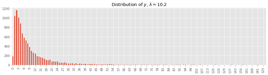
5.2. Visualize y

import matplotlib.pyplot as plt

plt.style.use('ggplot')

m = df['y'].mean()
s = df['y'].value_counts().sort_index()
ax = s.plot(kind='bar', figsize=(15, 3.5), title=rf'Distribution of $y$, $\lambda={m:.1f}$')
_ = ax.xaxis.set_major_locator(plt.MaxNLocator(50))

5.3. Poisson regression

from sklearn.linear_model import PoissonRegressor

X = df[df.columns.drop('y')]
y = df['y']

model = PoissonRegressor()
model.fit(X, y)

PoissonRegressor()

model.intercept_, model.coef_

(1.5793380835427167, array([0.44838229, 0.09694901]))

model.score(X, y)

0.20214296416305377

5.4. Histogram gradient boosting regression

We can use the experimental HistGradientBoostingRegressor algorithm.

from sklearn.experimental import enable_hist_gradient_boosting
from sklearn.ensemble import HistGradientBoostingRegressor

model = HistGradientBoostingRegressor(loss='poisson', max_leaf_nodes=64)
model.fit(X, y)

HistGradientBoostingRegressor(loss='poisson', max_leaf_nodes=64)

model.score(X, y)

0.41232578761756855