6. SHAP
SHAP’s goal is to explain machine learning output using a game theoretic approach. A primary use of SHAP is to understand how variables and values influence predictions visually and quantitatively. The API of SHAP is built along the explainers. These explainers are appropriate only for certain types or classes of algorithms. For example, you should use the TreeExplainer for tree-based models. Below, we take a look at three of these explainers.
Note that SHAP is a part of the movement to promote explanable artificial intelligence (AI). There are other APIs available that do similar things to SHAP.
A great book on explanable AI or interpretable machine learning is available online.
6.1. Linear explainer
The LinearExplainer is used to understand the outputs of linear predictors (e.g. linear regression). We will generate some data and use the LinearRegression model to learn the parameters from the data.
[1]:
%matplotlib inline
import numpy as np
import pandas as pd
from patsy import dmatrices
from numpy.random import normal
import matplotlib.pyplot as plt

np.random.seed(37)

n = 100

x_0 = normal(10, 1, n)
x_1 = normal(5, 2.5, n)
x_2 = normal(20, 1, n)
y = 3.2 + (2.7 * x_0) - (4.8 * x_1) + (1.3 * x_2) + normal(0, 1, n)

df = pd.DataFrame(np.hstack([
    x_0.reshape(-1, 1),
    x_1.reshape(-1, 1),
    x_2.reshape(-1, 1),
    y.reshape(-1, 1)]), columns=['x0', 'x1', 'x2', 'y'])

y, X = dmatrices('y ~ x0 + x1 + x2 - 1', df, return_type='dataframe')
print(f'X shape = {X.shape}, y shape {y.shape}')
X shape = (100, 3), y shape (100, 1)
[2]:
from sklearn.linear_model import LinearRegression

model = LinearRegression()
model.fit(X, y)
[2]:
LinearRegression()
Before you can use SHAP, you must initialize the JavaScript.
[3]:
import shap
from _runtime import SCIKIT_INTRO_CHECK_MODE, make_shap_classification_frame

def shap_select_class(values, class_index=1):
    if isinstance(values, list):
        return values[class_index]
    arr = np.asarray(values)
    if arr.ndim >= 3:
        return arr[..., class_index]
    return arr

def shap_select_expected_value(values, class_index=1):
    if isinstance(values, list):
        return values[class_index]
    arr = np.asarray(values)
    if arr.ndim == 0:
        return values
    return arr[class_index]

def shap_row(values, index):
    idx = min(index, len(values) - 1)
    return values[idx, :], idx

shap.initjs()

Here, we create the LinearExplainer. We have to pass in the dataset X.
[4]:
explainer = shap.LinearExplainer(model, X)
shap_values = explainer.shap_values(X)
A force plot can be used to explain each individual data point’s prediction. Below, we look at the force plots of the first, second and third observations (indexed 0, 1, 2).
First observation prediction explanation: the values of x1 and x2 are pushing the prediction value downard.
Second observation prediction explanation: the x0 value is pushing the prediction value higher, while x1 and x2 are pushing the value lower.
Third observation prediction explanation: the x0 and x1 values are pushing the prediction value lower and the x2 value is slightly nudging the value lower.
[5]:
shap.force_plot(explainer.expected_value, shap_values[0,:], X.iloc[0,:])
[5]:
Have you run `initjs()` in this notebook? If this notebook was from another user you must also trust this notebook (File -> Trust notebook). If you are viewing this notebook on github the Javascript has been stripped for security. If you are using JupyterLab this error is because a JupyterLab extension has not yet been written.
[6]:
shap.force_plot(explainer.expected_value, shap_values[1,:], X.iloc[1,:])
[6]:
Have you run `initjs()` in this notebook? If this notebook was from another user you must also trust this notebook (File -> Trust notebook). If you are viewing this notebook on github the Javascript has been stripped for security. If you are using JupyterLab this error is because a JupyterLab extension has not yet been written.
[7]:
shap.force_plot(explainer.expected_value, shap_values[2,:], X.iloc[2,:])
[7]:
Have you run `initjs()` in this notebook? If this notebook was from another user you must also trust this notebook (File -> Trust notebook). If you are viewing this notebook on github the Javascript has been stripped for security. If you are using JupyterLab this error is because a JupyterLab extension has not yet been written.
The force plot can also be used to visualize explanation over all observations.
[8]:
shap.force_plot(explainer.expected_value, shap_values, X)
[8]:
Have you run `initjs()` in this notebook? If this notebook was from another user you must also trust this notebook (File -> Trust notebook). If you are viewing this notebook on github the Javascript has been stripped for security. If you are using JupyterLab this error is because a JupyterLab extension has not yet been written.
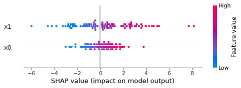
The summary plot is a way to understand variable importance.
[9]:
shap.summary_plot(shap_values, X)
Just for comparison, the visualization of the variables’ importance coincide with the coefficients of the linear regression model.
[10]:
s = pd.Series(model.coef_[0], index=X.columns)
s
[10]:
x0    2.536395
x1   -4.742098
x2    1.415208
dtype: float64
6.2. Tree explainer
The TreeExplainer is appropriate for algorithms using trees. Here, we generate data for a classification problem and use RandomForestClassifier as the model that we want to explain.
[11]:
df = make_shap_classification_frame(n_samples=20 if SCIKIT_INTRO_CHECK_MODE else 100)
X = df[['x0', 'x1']]
y = df.y
X shape = (100, 2), y shape (100, 1)
[12]:
from sklearn.ensemble import RandomForestClassifier
from _runtime import SCIKIT_INTRO_CHECK_MODE

model = RandomForestClassifier(n_estimators=20 if SCIKIT_INTRO_CHECK_MODE else 100, random_state=37)
model.fit(X, y.values.reshape(1, -1)[0])
[12]:
RandomForestClassifier(random_state=37)
[13]:
explainer = shap.TreeExplainer(model)
shap_values = explainer.shap_values(X)
shap_interaction_values = explainer.shap_interaction_values(X)
tree_expected_value = shap_select_expected_value(explainer.expected_value, 1)
tree_shap_values = shap_select_class(shap_values, 1)
tree_shap_interaction_values = shap_select_class(shap_interaction_values, 1)
Here are the forced plots for three observations.
[14]:
tree_row, tree_idx = shap_row(tree_shap_values, 0)
shap.force_plot(tree_expected_value, tree_row, X.iloc[tree_idx,:])
[14]:
Have you run `initjs()` in this notebook? If this notebook was from another user you must also trust this notebook (File -> Trust notebook). If you are viewing this notebook on github the Javascript has been stripped for security. If you are using JupyterLab this error is because a JupyterLab extension has not yet been written.
[15]:
tree_row, tree_idx = shap_row(tree_shap_values, 1)
shap.force_plot(tree_expected_value, tree_row, X.iloc[tree_idx,:])
[15]:
Have you run `initjs()` in this notebook? If this notebook was from another user you must also trust this notebook (File -> Trust notebook). If you are viewing this notebook on github the Javascript has been stripped for security. If you are using JupyterLab this error is because a JupyterLab extension has not yet been written.
[16]:
tree_row, tree_idx = shap_row(tree_shap_values, 95)
shap.force_plot(tree_expected_value, tree_row, X.iloc[tree_idx,:])
[16]:
Have you run `initjs()` in this notebook? If this notebook was from another user you must also trust this notebook (File -> Trust notebook). If you are viewing this notebook on github the Javascript has been stripped for security. If you are using JupyterLab this error is because a JupyterLab extension has not yet been written.
Here is the force plot for all observations.
[17]:
shap.force_plot(tree_expected_value, tree_shap_values, X)
[17]:
Have you run `initjs()` in this notebook? If this notebook was from another user you must also trust this notebook (File -> Trust notebook). If you are viewing this notebook on github the Javascript has been stripped for security. If you are using JupyterLab this error is because a JupyterLab extension has not yet been written.
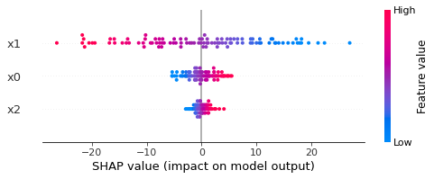
Below is the summary plot.
[18]:
shap.summary_plot(tree_shap_values, X)
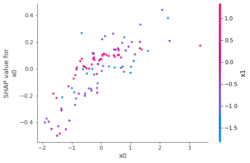
Below are dependence plots.
[19]:
shap.dependence_plot('x0', tree_shap_values, X)
[20]:
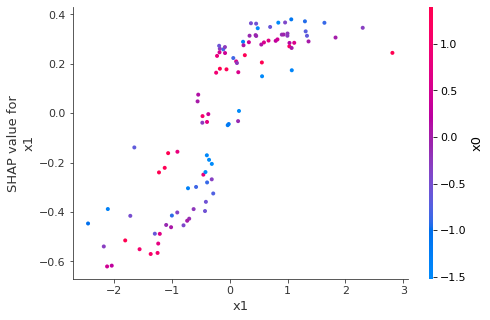
shap.dependence_plot('x1', tree_shap_values, X)
[21]:
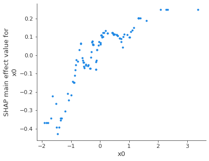
shap.dependence_plot(('x0', 'x0'), tree_shap_interaction_values, X)
[22]:
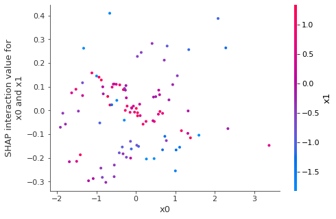
shap.dependence_plot(('x0', 'x1'), tree_shap_interaction_values, X)
[23]:
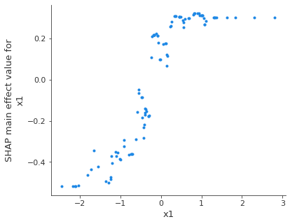
shap.dependence_plot(('x1', 'x1'), tree_shap_interaction_values, X)
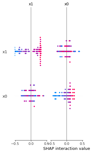
Lastly, the summary plot.
[24]:
shap.summary_plot(tree_shap_interaction_values, X)
6.3. Kernel explainer
The KernelExplainer is the general purpose explainer. Here, we use it to explain the LogisticRegression model. Notice the link parameter, which can be identity or logit. This argument specifies the model link to connect the feature importance values to the model output.
[25]:
from sklearn.linear_model import LogisticRegression

df = make_shap_classification_frame(n_samples=1000 if SCIKIT_INTRO_CHECK_MODE else 10000)
X = df[['x0', 'x1']]
y = df.y

model = LogisticRegression(fit_intercept=True, solver='saga', random_state=37)
model.fit(X, y.values.reshape(1, -1)[0])
[25]:
LogisticRegression(random_state=37, solver='saga')
[26]:
df = make_shap_classification_frame(n_samples=20 if SCIKIT_INTRO_CHECK_MODE else 100)
X = df[['x0', 'x1']]
y = df.y
Observe that we pass in the proababilistic prediction function to the KernelExplainer.
[27]:
explainer = shap.KernelExplainer(model.predict_proba, link='logit', data=X)
shap_values = explainer.shap_values(X)
kernel_expected_value = shap_select_expected_value(explainer.expected_value, 1)
kernel_shap_values = shap_select_class(shap_values, 1)
Again, example force plots on a few observations.
[28]:
kernel_row, kernel_idx = shap_row(kernel_shap_values, 0)
shap.force_plot(kernel_expected_value, kernel_row, X.iloc[kernel_idx,:], link='logit')
[28]:
Have you run `initjs()` in this notebook? If this notebook was from another user you must also trust this notebook (File -> Trust notebook). If you are viewing this notebook on github the Javascript has been stripped for security. If you are using JupyterLab this error is because a JupyterLab extension has not yet been written.
[29]:
kernel_row, kernel_idx = shap_row(kernel_shap_values, 1)
shap.force_plot(kernel_expected_value, kernel_row, X.iloc[kernel_idx,:], link='logit')
[29]:
Have you run `initjs()` in this notebook? If this notebook was from another user you must also trust this notebook (File -> Trust notebook). If you are viewing this notebook on github the Javascript has been stripped for security. If you are using JupyterLab this error is because a JupyterLab extension has not yet been written.
[30]:
kernel_row, kernel_idx = shap_row(kernel_shap_values, 99)
shap.force_plot(kernel_expected_value, kernel_row, X.iloc[kernel_idx,:], link='logit')
[30]:
Have you run `initjs()` in this notebook? If this notebook was from another user you must also trust this notebook (File -> Trust notebook). If you are viewing this notebook on github the Javascript has been stripped for security. If you are using JupyterLab this error is because a JupyterLab extension has not yet been written.
The force plot over all observations.
[31]:
shap.force_plot(kernel_expected_value, kernel_shap_values, X, link='logit')
[31]:
Have you run `initjs()` in this notebook? If this notebook was from another user you must also trust this notebook (File -> Trust notebook). If you are viewing this notebook on github the Javascript has been stripped for security. If you are using JupyterLab this error is because a JupyterLab extension has not yet been written.
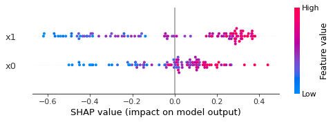
Lastly, the summary plot.
[32]:
shap.summary_plot(kernel_shap_values, X)