5. statsmodels

statsmodel is another statistical library you may use to get more information on your regression models. Let’s take a look at how to do some simple things with this API. Below, we create functions to get data for regression and classification.

%matplotlib inline
import matplotlib.pyplot as plt
from sklearn.datasets import make_regression, make_classification
import numpy as np
import pandas as pd

np.random.seed(37)
plt.style.use('ggplot')

def get_regression_data(n_features=5, n_samples=1000):
    X, y = make_regression(**{
        'n_samples': n_samples,
        'n_features': n_features,
        'n_informative': n_features,
        'n_targets': 1,
        'bias': 5.3,
        'random_state': 37
    })

    data = np.hstack([X, y.reshape(-1, 1)])
    cols = [f'x{i}' for i in range(n_features)] + ['y']
    return pd.DataFrame(data, columns=cols)

def get_classification_data(n_features=5, n_samples=1000):
    X, y = make_classification(**{
        'n_samples': n_samples,
        'n_features': n_features,
        'n_informative': n_features,
        'n_redundant': 0,
        'n_repeated': 0,
        'n_classes': 2,
        'n_clusters_per_class': 1,
        'random_state': 37
    })

    data = np.hstack([X, y.reshape(-1, 1)])
    cols = [f'x{i}' for i in range(n_features)] + ['y']
    return pd.DataFrame(data, columns=cols)

5.1. Ordinary least square

An ordinary least square (OLS) model is created using the OLS() function. Below, the patsy API is used to separate the dataframe using R style equation syntax.

import statsmodels.api as sm
from patsy import dmatrices

df = get_regression_data()
y, X = dmatrices('y ~ x0 + x1 + x2 + x3 + x4', data=df, return_type='dataframe')
mod = sm.OLS(y, X)
res = mod.fit()

You can also bypass patsy and use the formula API to define the model.

import statsmodels.formula.api as smf

mod = smf.ols(formula='y ~ x0 + x1 + x2 + x3 + x4', data=df)
res = mod.fit()

The summary of the data is available through summary().

res.summary()

OLS Regression Results

Dep. Variable:	y	R-squared:	1.000
Model:	OLS	Adj. R-squared:	1.000
Method:	Least Squares	F-statistic:	7.399e+32
Date:	Tue, 01 Dec 2020	Prob (F-statistic):	0.00
Time:	17:09:02	Log-Likelihood:	29657.
No. Observations:	1000	AIC:	-5.930e+04
Df Residuals:	994	BIC:	-5.927e+04
Df Model:	5
Covariance Type:	nonrobust

	coef	std err	t	P>|t|	[0.025	0.975]
Intercept	5.3000	1.01e-15	5.23e+15	0.000	5.300	5.300
x0	41.8134	1.02e-15	4.1e+16	0.000	41.813	41.813
x1	25.0388	1.08e-15	2.33e+16	0.000	25.039	25.039
x2	3.2108	1.02e-15	3.14e+15	0.000	3.211	3.211
x3	29.9942	1.01e-15	2.98e+16	0.000	29.994	29.994
x4	25.3606	1e-15	2.53e+16	0.000	25.361	25.361

Omnibus:	7.219	Durbin-Watson:	1.895
Prob(Omnibus):	0.027	Jarque-Bera (JB):	8.934
Skew:	0.086	Prob(JB):	0.0115
Kurtosis:	3.430	Cond. No.	1.16

Notes:
[1] Standard Errors assume that the covariance matrix of the errors is correctly specified.

The params properties of the results will retrieve the coefficients of the model.

res.params

Intercept     5.300000
x0           41.813417
x1           25.038808
x2            3.210812
x3           29.994205
x4           25.360629
dtype: float64

The rsquared property will retrieve the \(R^2\) value.

res.rsquared

1.0

There are a lot of model diagnostic functions available. Below, we apply the rainbow test for linearity.

f_stats, p_value = sm.stats.linear_rainbow(res)
print(f'f-statistic: {f_stats:.5f}, p-value: {p_value:.5f}')

f-statistic: 0.24804, p-value: 1.00000

5.2. Logistic regression

Logistic regression is a type of generalized linear model. A logistic regression model is created using the GLM() function. Note that y comes before X for GLM(), as opposed to X coming before y when using OLS().

df = get_classification_data()
y, X = dmatrices('y ~ x0 + x1 + x2 + x3 + x4', data=df, return_type='dataframe')
binonmial_model = sm.GLM(y, X, family=sm.families.Binomial())
res = binonmial_model.fit()

res.summary()

Generalized Linear Model Regression Results

Dep. Variable:	y	No. Observations:	1000
Model:	GLM	Df Residuals:	994
Model Family:	Binomial	Df Model:	5
Link Function:	logit	Scale:	1.0000
Method:	IRLS	Log-Likelihood:	-76.314
Date:	Tue, 01 Dec 2020	Deviance:	152.63
Time:	17:09:02	Pearson chi2:	9.15e+05
No. Iterations:	9
Covariance Type:	nonrobust

	coef	std err	z	P>|z|	[0.025	0.975]
Intercept	-1.5205	0.636	-2.389	0.017	-2.768	-0.273
x0	2.2090	0.259	8.522	0.000	1.701	2.717
x1	-3.1632	0.348	-9.083	0.000	-3.846	-2.481
x2	2.0077	0.248	8.095	0.000	1.522	2.494
x3	-1.0259	0.301	-3.408	0.001	-1.616	-0.436
x4	2.6748	0.382	7.010	0.000	1.927	3.423

5.3. ANOVA

Analysis of Variance (ANOVA) may be conducted. The data below is taken from here.

df = pd.DataFrame({
    'A': [25, 30, 28, 36, 29],
    'B': [45, 55, 29, 56, 40],
    'C': [30, 29, 33, 37, 27],
    'D': [54, 60, 51, 62, 73]
})
df

	A	B	C	D
0	25	45	30	54
1	30	55	29	60
2	28	29	33	51
3	36	56	37	62
4	29	40	27	73

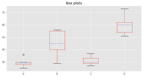
Let’s do some box plots.

fig, ax = plt.subplots(figsize=(10, 5))

_ = df.plot(kind='box', ax=ax)
_ = ax.set_title('Box plots')

scipy can do the one-way ANOVA.

import scipy.stats as stats

f, p = stats.f_oneway(*[df[c] for c in df.columns])
print(f'f-statistics: {f:.5f}, p-value: {p:.5f}')

f-statistics: 17.49281, p-value: 0.00003

Before statsmodel can do ANOVA, we have to melt the dataframe.

ldf = pd.melt(df.reset_index(), id_vars=['index'], value_vars=['A', 'B', 'C', 'D'])\
    .rename(columns={'index': 'index', 'variable': 'treatment', 'value': 'value'})
ldf.head()

	index	treatment	value
0	0	A	25
1	1	A	30
2	2	A	28
3	3	A	36
4	4	A	29

Now we specify the ANOVA model and acquire the table.

anova_model = smf.ols('value ~ C(treatment)', data=ldf).fit()
anova_table = sm.stats.anova_lm(anova_model, typ=2)
anova_table

	sum_sq	df	F	PR(>F)
C(treatment)	3010.95	3.0	17.49281	0.000026
Residual	918.00	16.0	NaN	NaN

Post-hoc testing is also possible.

from statsmodels.stats.multicomp import pairwise_tukeyhsd

res = pairwise_tukeyhsd(ldf.value, ldf.treatment)
res.summary()

Multiple Comparison of Means - Tukey HSD, FWER=0.05

group1	group2	meandiff	p-adj	lower	upper	reject
A	B	15.4	0.0251	1.6929	29.1071	True
A	C	1.6	0.9	-12.1071	15.3071	False
A	D	30.4	0.001	16.6929	44.1071	True
B	C	-13.8	0.0482	-27.5071	-0.0929	True
B	D	15.0	0.0296	1.2929	28.7071	True
C	D	28.8	0.001	15.0929	42.5071	True