7. imbalanced-learn
imbalanced-learn is a package to deal with imbalance in data. The data imbalance typically manifest when you have data with class labels, and one or more of these classes suffers from having too few examples to learn from. imbalanced-learn has three broad categories of approaches to deal with class imbalance.
oversampling: oversample the minority class
understampling: undersample the majority class
combination: use a combination of oversampling and undersampling
Let’s investigate the use of each of these approaches in dealing with the class imbalance problem.
7.1. Data generation
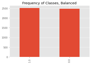
Here, we will create a dataset using Scikit-Learn’s make_classification() method. There will be only 2 classes, and as you will see, the samples per class that are about the same amount.
[1]:
import matplotlib.pyplot as plt
from sklearn.datasets import make_classification
import numpy as np
import pandas as pd

plt.style.use('ggplot')
np.random.seed(37)

X, y = make_classification(**{
    'n_samples': 5000,
    'n_features': 5,
    'n_classes': 2,
    'random_state': 37
})

columns = [f'x{i}' for i in range(X.shape[1])] + ['y']
df = pd.DataFrame(np.hstack([X, y.reshape(-1, 1)]), columns=columns)

print(df.shape)
(5000, 6)
[2]:
df.head()
[2]:
| x0 | x1 | x2 | x3 | x4 | y | |
|---|---|---|---|---|---|---|
| 0 | -0.729402 | 0.390517 | -0.603771 | 0.286312 | -0.266412 | 0.0 |
| 1 | 0.030495 | -0.970299 | 1.223902 | -0.343972 | -0.479884 | 0.0 |
| 2 | -0.657696 | -0.811643 | -1.075159 | 0.405169 | -0.022806 | 0.0 |
| 3 | 0.138540 | 2.012018 | -1.825350 | 0.482964 | 0.845321 | 1.0 |
| 4 | 2.231350 | -0.705512 | -0.453736 | -0.238611 | 1.757486 | 1.0 |
[3]:
ax = df.y.value_counts().plot(kind='bar')
_ = ax.set_title('Frequency of Classes, Balanced')
7.2. Class imbalance
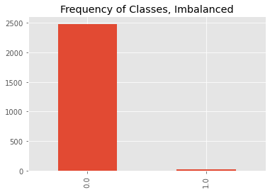
We will then transform the data so that class 0 is the majority class and class 1 is the minority class. Class 1 will have only 1% of what was originally generated.
[4]:
df0 = df[df.y == 0].copy(deep=True).reset_index(drop=True)
df1 = df[df.y == 1].sample(frac=0.01).copy(deep=True).reset_index(drop=True)

df = pd.concat([df0, df1])
[5]:
df.shape
[5]:
(2508, 6)
[6]:
ax = df.y.value_counts().plot(kind='bar')
_ = ax.set_title('Frequency of Classes, Imbalanced')
7.3. Learning with class imbalance
We will use a random forest classifier to learn from the imbalanced data. The learning will be validated using a stratified k=10 fold approach. We will also benchmark the performance of the random forest classifier using Area Under the Curve (auc) and Average Precision Score (aps).
[7]:
X = df[[c for c in df.columns if c != 'y']]
y = df.y

print(X.shape, y.shape)
(2508, 5) (2508,)
[8]:
from sklearn.model_selection import StratifiedKFold
from sklearn.linear_model import LogisticRegression
from sklearn.ensemble import RandomForestClassifier
from sklearn.metrics import roc_auc_score, average_precision_score

skf = StratifiedKFold(n_splits=10, shuffle=True, random_state=37)

rdf = []
for fold, (tr, te) in enumerate(skf.split(X, y)):
    X_tr, X_te = X.iloc[tr], X.iloc[te]
    y_tr, y_te = y.iloc[tr], y.iloc[te]

    model = LogisticRegression(penalty='l2', solver='liblinear', random_state=37)
    model = RandomForestClassifier(n_jobs=-1, random_state=37)
    model.fit(X_tr, y_tr)
    y_pr = model.predict_proba(X_te)[:,1]

    auc = roc_auc_score(y_te, y_pr)
    aps = average_precision_score(y_te, y_pr)

    rdf.append({'auc': auc, 'aps': aps})

rdf = pd.DataFrame(rdf)
[9]:
rdf[['auc', 'aps']].agg(['mean', 'std'])
[9]:
| auc | aps | |
|---|---|---|
| mean | 0.972218 | 0.750400 |
| std | 0.080609 | 0.305972 |
7.4. Oversampling
Below are the results of applying multiple oversampling techniques with random forest classification validated by stratified, k-fold cross-validation.
[10]:
from imblearn.over_sampling import RandomOverSampler, SMOTE, ADASYN, BorderlineSMOTE, SVMSMOTE, KMeansSMOTE
from sklearn.cluster import KMeans
from collections import Counter
from itertools import chain

def get_oversampler(sampler):
    if 'adasyn' == sampler:
        p = {
            'random_state': 37,
            'n_neighbors': 5
        }
        return ADASYN(**p)
    elif 'borderlinesmote' == sampler:
        p = {
            'random_state': 37,
            'k_neighbors': 5,
            'm_neighbors': 10
        }
        return BorderlineSMOTE(**p)
    elif 'svmsmote' == sampler:
        p = {
            'random_state': 37,
            'k_neighbors': 5,
            'm_neighbors': 10
        }
        return SVMSMOTE(**p)
    elif 'kmeanssmote' == sampler:
        kmeans = KMeans(n_clusters=5, random_state=37)
        p = {
            'random_state': 37,
            'k_neighbors': 5,
            'kmeans_estimator': kmeans
        }
        return KMeansSMOTE(**p)
    elif 'random' == sampler:
        p = {
            'random_state': 37
        }
        return RandomOverSampler(**p)
    else:
        p = {
            'random_state': 37,
            'k_neighbors': 5
        }
        return SMOTE(**p)

def get_results(sampler, f):
    skf = StratifiedKFold(n_splits=10, shuffle=True, random_state=37)

    results = []
    for fold, (tr, te) in enumerate(skf.split(X, y)):
        X_tr, X_te = X.iloc[tr], X.iloc[te]
        y_tr, y_te = y.iloc[tr], y.iloc[te]

        counts = sorted(Counter(y_tr).items())
        n_0, n_1 = counts[0][1], counts[1][1]

        if sampler != 'none':
            sampling_approach = f(sampler)
            X_tr, y_tr = sampling_approach.fit_resample(X_tr, y_tr)

        model = RandomForestClassifier(n_jobs=-1, random_state=37)
        model.fit(X_tr, y_tr)
        y_pr = model.predict_proba(X_te)[:,1]

        auc = roc_auc_score(y_te, y_pr)
        aps = average_precision_score(y_te, y_pr)

        counts = sorted(Counter(y_tr).items())
        r_0, r_1 = counts[0][1], counts[1][1]

        results.append({
            'sampler': sampler,
            'auc': auc,
            'aps': aps,
            'n_maj': n_0,
            'r_maj': r_0,
            'n_min': n_1,
            'r_min': r_1
        })

    return results
[11]:
%%time

samplers = ['none', 'random', 'smote', 'adasyn', 'borderlinesmote', 'svmsmote']
odf = pd.DataFrame(list(chain(*[get_results(s, get_oversampler) for s in samplers])))
Wall time: 15 s
[12]:
odf[['sampler', 'auc', 'aps']].groupby('sampler').agg(['mean', 'std'])
[12]:
| auc | aps | |||
|---|---|---|---|---|
| mean | std | mean | std | |
| sampler | ||||
| adasyn | 0.971713 | 0.080083 | 0.748178 | 0.222613 |
| borderlinesmote | 0.971511 | 0.080007 | 0.734289 | 0.206186 |
| none | 0.972218 | 0.080609 | 0.750400 | 0.305972 |
| random | 0.972351 | 0.079962 | 0.778178 | 0.242363 |
| smote | 0.972014 | 0.079815 | 0.759844 | 0.204722 |
| svmsmote | 0.971881 | 0.080504 | 0.739844 | 0.278877 |
7.5. Undersampling
Below are the results of applying multiple undersampling techniques with random forest classification validated by stratified, k-fold cross-validation.
[13]:
from imblearn.under_sampling import RandomUnderSampler, NearMiss, EditedNearestNeighbours, RepeatedEditedNearestNeighbours, CondensedNearestNeighbour, OneSidedSelection, NeighbourhoodCleaningRule, InstanceHardnessThreshold

def get_undersampler(sampler):
    if 'random' == sampler:
        p = {
            'random_state': 37
        }
        return RandomUnderSampler(**p)
    elif 'nearmiss1' == sampler:
        p = {
            'version': 1
        }
        return NearMiss(**p)
    elif 'nearmiss2' == sampler:
        p = {
            'version': 2
        }
        return NearMiss(**p)
    elif 'nearmiss3' == sampler:
        p = {
            'version': 3
        }
        return NearMiss(**p)
    elif 'editednn' == sampler:
        return EditedNearestNeighbours()
    elif 'reditednn' == sampler:
        return RepeatedEditedNearestNeighbours()
    elif 'condensednn' == sampler:
        p = {
            'random_state': 37
        }
        return CondensedNearestNeighbour(**p)
    elif 'onesided' == sampler:
        p = {
            'random_state': 37
        }
        return OneSidedSelection(**p)
    elif 'neighcleanrule' == sampler:
        return NeighbourhoodCleaningRule()
    elif 'instancehardthresh' == sampler:
        estimator = LogisticRegression(solver='lbfgs', multi_class='auto')
        p = {
            'estimator': estimator,
            'random_state': 37
        }
        return InstanceHardnessThreshold(**p)
[14]:
%%time

samplers = ['random', 'nearmiss1', 'nearmiss2',
            'nearmiss3', 'editednn', 'reditednn', 'condensednn',
            'onesided', 'neighcleanrule']
udf = pd.DataFrame(list(chain(*[get_results(s, get_undersampler) for s in samplers])))
Wall time: 48.4 s
[15]:
udf[['sampler', 'auc', 'aps']].groupby('sampler').agg(['mean', 'std'])
[15]:
| auc | aps | |||
|---|---|---|---|---|
| mean | std | mean | std | |
| sampler | ||||
| condensednn | 0.994261 | 0.010101 | 0.746438 | 0.278687 |
| editednn | 0.971847 | 0.081873 | 0.745956 | 0.281920 |
| nearmiss1 | 0.991982 | 0.007731 | 0.661993 | 0.202126 |
| nearmiss2 | 0.992929 | 0.009534 | 0.678327 | 0.251700 |
| nearmiss3 | 0.991876 | 0.015964 | 0.727037 | 0.274334 |
| neighcleanrule | 0.972518 | 0.081746 | 0.808733 | 0.265511 |
| onesided | 0.971445 | 0.082091 | 0.714289 | 0.278155 |
| random | 0.996172 | 0.006600 | 0.792222 | 0.225959 |
| reditednn | 0.972047 | 0.081932 | 0.767622 | 0.258529 |
7.6. Combination
Below are the results of applying multiple combination techniques with random forest classification validated by stratified, k-fold cross-validation.
[16]:
from imblearn.combine import SMOTEENN, SMOTETomek

def get_combine(sampler):
    if 'smoteenn' == sampler:
        p = {
            'random_state': 37,
            'k_neighbors': 5
        }
        smote = SMOTE(**p)

        enn = EditedNearestNeighbours()

        p = {
            'smote': smote,
            'enn': enn,
            'random_state': 37
        }
        return SMOTEENN(**p)
    elif 'smotetomek' == sampler:
        p = {
            'random_state': 37,
            'k_neighbors': 5
        }
        smote = SMOTE(**p)

        p = {
            'smote': smote,
            'random_state': 37
        }
        return SMOTETomek(**p)
[17]:
%%time

samplers = ['smoteenn', 'smotetomek']
cdf = pd.DataFrame(list(chain(*[get_results(s, get_combine) for s in samplers])))
Wall time: 5.35 s
[18]:
cdf[['sampler', 'auc', 'aps']].groupby('sampler').agg(['mean', 'std'])
[18]:
| auc | aps | |||
|---|---|---|---|---|
| mean | std | mean | std | |
| sampler | ||||
| smoteenn | 0.971678 | 0.080401 | 0.726511 | 0.241162 |
| smotetomek | 0.972014 | 0.079815 | 0.759844 | 0.204722 |
7.7. Comparisons
Here, we will compare the results of all sampling approaches.
[19]:
odf['type'] = odf.sampler.apply(lambda s: 'baseline' if s == 'none' else 'over')
udf['type'] = 'under'
cdf['type'] = 'combo'

rdf = pd.concat([odf, udf, cdf]).reset_index(drop=True)
As you can see below,
all sampling techniques do about the same in terms of
AUC,the differences is with the
APSperformance,undersampling with neighborhood cleaning rule seems to do the best, and
surprisingly, no sampling is still competitive.
[20]:
sort = [('aps', 'mean'), ('aps', 'std'), ('auc', 'mean'), ('auc', 'std')]
rdf[['sampler', 'type', 'auc', 'aps']]\
    .groupby(['type', 'sampler'])\
    .agg(['mean', 'std'])\
    .sort_values(sort, ascending=False)
[20]:
| auc | aps | ||||
|---|---|---|---|---|---|
| mean | std | mean | std | ||
| type | sampler | ||||
| under | neighcleanrule | 0.972518 | 0.081746 | 0.808733 | 0.265511 |
| random | 0.996172 | 0.006600 | 0.792222 | 0.225959 | |
| over | random | 0.972351 | 0.079962 | 0.778178 | 0.242363 |
| under | reditednn | 0.972047 | 0.081932 | 0.767622 | 0.258529 |
| combo | smotetomek | 0.972014 | 0.079815 | 0.759844 | 0.204722 |
| over | smote | 0.972014 | 0.079815 | 0.759844 | 0.204722 |
| baseline | none | 0.972218 | 0.080609 | 0.750400 | 0.305972 |
| over | adasyn | 0.971713 | 0.080083 | 0.748178 | 0.222613 |
| under | condensednn | 0.994261 | 0.010101 | 0.746438 | 0.278687 |
| editednn | 0.971847 | 0.081873 | 0.745956 | 0.281920 | |
| over | svmsmote | 0.971881 | 0.080504 | 0.739844 | 0.278877 |
| borderlinesmote | 0.971511 | 0.080007 | 0.734289 | 0.206186 | |
| under | nearmiss3 | 0.991876 | 0.015964 | 0.727037 | 0.274334 |
| combo | smoteenn | 0.971678 | 0.080401 | 0.726511 | 0.241162 |
| under | onesided | 0.971445 | 0.082091 | 0.714289 | 0.278155 |
| nearmiss2 | 0.992929 | 0.009534 | 0.678327 | 0.251700 | |
| nearmiss1 | 0.991982 | 0.007731 | 0.661993 | 0.202126 | |
7.8. Pipeline
If you need to use one of the samplers in a pipeline, do not use sklearn.pipeline.Pipeline, instead, use imblearn.pipeline, which is a drop-in replacement. Here’s an example of a learning pipeline with hyperparameter tuning.
[21]:
from imblearn.pipeline import Pipeline
from sklearn.ensemble import RandomForestClassifier
from sklearn.metrics import roc_auc_score, average_precision_score, make_scorer
from sklearn.model_selection import StratifiedKFold, GridSearchCV
from sklearn.preprocessing import MinMaxScaler
from _runtime import SCIKIT_INTRO_CHECK_MODE

def get_model(n_splits=None):
    n_splits = n_splits or (2 if SCIKIT_INTRO_CHECK_MODE else 5)
    cv = StratifiedKFold(**{
        'n_splits': n_splits,
        'shuffle': True,
        'random_state': 37
    })

    auc_scorer = make_scorer(
        roc_auc_score,
        greater_is_better=True,
        response_method='predict_proba',
        multi_class='ovo')

    scoring = {
      'auc': auc_scorer
    }

    scaler = MinMaxScaler()
    sampler = ADASYN(**{
        'random_state': 37
    })
    classifier = RandomForestClassifier(**{
        'random_state': 37,
        'n_jobs': 1 if SCIKIT_INTRO_CHECK_MODE else -1,
        'verbose': 0
    })

    pipeline = Pipeline([
        ('scaler', scaler),
        ('sampler', sampler),
        ('classifier', classifier)
    ])

    param_grid = {
      'sampler__sampling_strategy': ['auto'] if SCIKIT_INTRO_CHECK_MODE else ['all', 'auto'],
      'sampler__n_neighbors': [3] if SCIKIT_INTRO_CHECK_MODE else [3, 5],
      'classifier__n_estimators': [25] if SCIKIT_INTRO_CHECK_MODE else [50, 100]
    }

    model = GridSearchCV(**{
        'estimator': pipeline,
        'cv': cv,
        'param_grid': param_grid,
        'verbose': 0 if SCIKIT_INTRO_CHECK_MODE else 1,
        'scoring': scoring,
        'refit': 'auc',
        'error_score': np.nan,
        'n_jobs': 1 if SCIKIT_INTRO_CHECK_MODE else -1
    })
    return model
[22]:
model = get_model(n_splits=2)
model.fit(X, y)
Fitting 2 folds for each of 8 candidates, totalling 16 fits
[Parallel(n_jobs=-1)]: Using backend LokyBackend with 16 concurrent workers.
[Parallel(n_jobs=-1)]: Done   2 out of  16 | elapsed:    3.8s remaining:   27.4s
[Parallel(n_jobs=-1)]: Done  16 out of  16 | elapsed:    4.2s finished
[22]:
GridSearchCV(cv=StratifiedKFold(n_splits=2, random_state=37, shuffle=True),
             estimator=Pipeline(steps=[('scaler', MinMaxScaler()),
                                       ('sampler',
                                        ADASYN(n_jobs=-1, random_state=37)),
                                       ('classifier',
                                        RandomForestClassifier(n_jobs=-1,
                                                               random_state=37))]),
             n_jobs=-1,
             param_grid={'classifier__n_estimators': [50, 100],
                         'sampler__n_neighbors': [3, 5],
                         'sampler__sampling_strategy': ['all', 'auto']},
             refit='auc',
             scoring={'auc': make_scorer(roc_auc_score, needs_proba=True, multi_class=ovo)},
             verbose=1)
[23]:
model.best_params_
[23]:
{'classifier__n_estimators': 100,
 'sampler__n_neighbors': 3,
 'sampler__sampling_strategy': 'all'}
[24]:
y_pr = model.predict_proba(X)[:,1]

auc = roc_auc_score(y, y_pr)
aps = average_precision_score(y, y_pr)

print(f'auc = {auc:.5f}, aps = {aps:.5f}')
auc = 1.00000, aps = 1.00000